2 Mathematical Foundations
Finite element analysis uses ideas from linear algebra, tensor calculus, and functional analysis. Students often encounter these subjects separately. This chapter collects the concepts needed to formulate boundary-value problems and their finite element approximations in a consistent notation. The treatment is selective and assumes only multivariable calculus and elementary linear algebra. Additional details related to real analysis and tensor and continuum mechanics concepts used in this chapter can be found in Appendix A and Appendix B.
2.1 Sets and basic notation
A set is a collection of distinct objects. The objects in a set are its elements. Curly braces \(\{\,\}\) are used to specify which elements belong to the set. For example,
\[ A=\{1,2,3\} \]
defines the set whose elements are \(1\), \(2\), and \(3\). We write \(2\in A\) to state that \(2\) belongs to \(A\), and \(4\notin A\) to state that \(4\) does not belong to \(A\). The order and repetition of listed elements do not matter:
\[ \{1,2,3\}=\{3,2,1\}=\{1,1,2,3\}. \]
Two sets are equal when they have exactly the same elements. An element and a set containing that element are different objects. For example, \(1\in\{1\}\), but \(1\ne\{1\}\).
When listing every element is inconvenient or impossible, we use set-builder notation. The general form
\[ \{x\in X:P(x)\} \]
means “the set of all elements \(x\) of \(X\) for which the condition \(P(x)\) is true.” The colon is read as “such that.” A vertical bar is sometimes used in place of the colon. For example,
\[ \{x\in\R:x^2<4\}=(-2,2), \]
because the real numbers satisfying \(x^2<4\) are precisely those between \(-2\) and \(2\). Similarly,
\[ \{(x,y)\in\R^2:y=x\} \]
is the line through the origin with slope one. The expression to the left of the colon identifies the objects under consideration; the expression to the right gives the condition those objects must satisfy.
A set \(A\) is a subset of a set \(B\), written \(A\subset B\), if every element of \(A\) also belongs to \(B\). In this book, \(A\subset B\) allows the possibility that \(A=B\); a strict subset is written \(A\subsetneq B\). The set with no elements is the empty set, denoted by \(\varnothing\).
For two sets \(A\) and \(B\),
\[ \begin{aligned} A\cup B &=\{x:x\in A\text{ or }x\in B\},\\ A\cap B &=\{x:x\in A\text{ and }x\in B\},\\ A\setminus B &=\{x\in A:x\notin B\}. \end{aligned} \]
These are the union, intersection, and set difference, respectively. The Cartesian product is
\[ A\times B=\{(a,b):a\in A\text{ and }b\in B\}. \]
Thus \(\R^2=\R\times\R\), and more generally \(\R^d\) is the set of ordered \(d\)-tuples of real numbers.
Intervals are sets of real numbers. For \(a<b\),
\[ (a,b)=\{x\in\R:a<x<b\}, \qquad [a,b]=\{x\in\R:a\leq x\leq b\}. \]
The first interval excludes its endpoints and the second includes them.
The standard number sets used in this chapter are
\[ \mathbb{N}=\{0,1,2,\ldots\}, \qquad \mathbb{Z}=\{\ldots,-2,-1,0,1,2,\ldots\}, \qquad \mathbb{Q}\subset\R, \]
where \(\mathbb{N}\), \(\mathbb{Z}\), \(\mathbb{Q}\), and \(\R\) denote the natural numbers, integers, rational numbers, and real numbers, respectively.
A function \(f:X\to Y\) assigns one element \(f(x)\in Y\) to each \(x\in X\). The set \(X\) is the domain of the function and \(Y\) is its codomain. The braces used to describe a set specify only its elements; they do not, by themselves, define vector addition, scalar multiplication, a metric, or a norm.
Exercise 2.1 (Reading and writing sets)
- List the elements of \(A=\{n\in\mathbb{N}:0\leq n\leq4\}\).
- Write the interval \([-1,2)\) in set-builder notation.
- Let \(B=\{x\in\R:x^2=1\}\). List the elements of \(B\) and determine whether \(B\subset[-1,1]\).
- List the ordered pairs in \(\{0,1\}\times\{2,3\}\).
- Describe \(\{(x,y)\in\R^2:y=2x\}\) in words and determine whether \((2,4)\) and \((2,5)\) belong to this set.
2.2 Domains and boundary regularity
Throughout the book, \(\Om\subset\R^d\) denotes a nonempty, connected, open set. Unless stated otherwise, \(\Om\) is also bounded. Its closure and boundary are denoted by \(\overline{\Om}\) and \(\partial\Om\), respectively. Additional regularity of the boundary will be stated when it is needed.
Definition 2.1 (Lipschitz domain) A bounded domain \(\Om\subset\R^d\) is a Lipschitz domain if, near every point of \(\partial\Om\), its boundary can be represented as the graph of a Lipschitz-continuous function after a translation and rotation of coordinates. More precisely, for every \(\bx_0\in\partial\Om\), there are a neighborhood \(U\) of \(\bx_0\), local coordinates \((\bx',x_d)\in\R^{d-1}\times\R\), and a function \(\varphi:\R^{d-1}\to\R\) such that
\[ \Om\cap U =\{(\bx',x_d)\in U:x_d>\varphi(\bx')\}, \]
with the opposite inequality allowed after reversing the \(x_d\)-axis. The function \(\varphi\) is Lipschitz continuous if there is a constant \(L>0\) such that
\[ |\varphi(\bx')-\varphi(\bm{y}')| \leq L\norm{\bx'-\bm{y}'}_2 \qquad \forall\bx',\bm{y}'\in\R^{d-1}. \]
Here \(\norm{\bm{z}}_2=(\sum_{i=1}^{d-1}z_i^2)^{1/2}\) is the Euclidean norm of \(\bm{z}\in\R^{d-1}\).
Example 2.1 (Common domains)
- An open interval \((a,b)\subset\R\) is a bounded Lipschitz domain.
- Open rectangles, polygons, boxes, and polyhedra with non-self-intersecting boundaries are Lipschitz domains. Corners and reentrant corners are permitted; the L-shaped domain \((-1,1)^2\setminus([0,1)\times(-1,0])\) is a standard example.
- The open ball \(\{\bx\in\R^d:\norm{\bx}_2<R\}\) has a smooth boundary and is therefore a Lipschitz domain.
Remark 2.1 (Use of domain assumptions). The fine distinctions among boundary regularity classes are not a main topic of this book. When a result requires a Lipschitz boundary, a positive-measure Dirichlet boundary, or another geometric property, that condition will be assumed at the outset. These assumptions allow us to assign boundary values to \(H^1\) functions, use outward unit normals, apply integration by parts, and use Poincare-type inequalities without interrupting the finite element development with additional technical proofs.
2.3 Scalars, vectors, and tensors
A scalar is a real number. Scalars describe quantities that have a value but no direction. Temperature, density, and isotropic thermal conductivity are examples. A scalar field assigns a scalar to each point of a domain; for example, a temperature field is a function \(T:\Om\to\R\).
A vector describes a quantity with components along spatial directions. Displacement, traction, velocity, and heat flux are vector fields. At each point \(\bx\in\Om\), a vector field \(\bm{a}:\Om\to\R^d\) assigns a vector \(\bm{a}(\bx)\). Before working with vector and tensor components, we must specify the coordinate directions with respect to which those components are measured.
2.3.1 Cartesian coordinates and vector components
A Cartesian coordinate system in \(\R^d\) consists of an origin and an orthonormal basis
\[ \{\bm{e}_1,\ldots,\bm{e}_d\}. \]
The basis vectors have unit length and are mutually perpendicular. Their dot products satisfy
\[ \bm{e}_i\cdot\bm{e}_j=\delta_{ij}, \qquad \delta_{ij}= \begin{cases} 1, & i=j,\\ 0, & i\ne j, \end{cases} \tag{2.1}\]
where \(\delta_{ij}\) is the Kronecker delta. In \(\R^2\), the usual Cartesian basis is \(\bm{e}_1=(1,0)\) and \(\bm{e}_2=(0,1)\); in \(\R^3\), it is \(\bm{e}_1=(1,0,0)\), \(\bm{e}_2=(0,1,0)\), and \(\bm{e}_3=(0,0,1)\).
Every vector \(\bm{a}\in\R^d\) has a unique expansion
\[ \bm{a} =a_1\bm{e}_1+\cdots+a_d\bm{e}_d =a_i\bm{e}_i. \tag{2.2}\]
The scalar \(a_i\) is the component of \(\bm{a}\) in the \(\bm{e}_i\) direction. Taking the dot product of Equation 2.2 with \(\bm{e}_j\) gives
\[ \bm{a}\cdot\bm{e}_j =a_i(\bm{e}_i\cdot\bm{e}_j) =a_i\delta_{ij} =a_j. \]
Thus the components can be recovered from the vector by \(a_i=\bm{a}\cdot\bm{e}_i\). The vector is the geometric object, whereas the list of components \((a_1,\ldots,a_d)\) describes that vector in the selected basis.
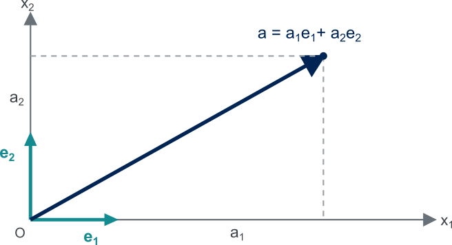
For vectors \(\bm{a}=a_i\bm{e}_i\) and \(\bm{b}=b_i\bm{e}_i\), orthonormality gives
\[ \bm{a}\cdot\bm{b}=a_i b_i, \qquad \lVert\bm{a}\rVert =\sqrt{\bm{a}\cdot\bm{a}} =\left(\sum_{i=1}^d a_i^2\right)^{1/2}. \tag{2.3}\]
Example 2.2 (Components of a vector in \(\R^3\)) Let
\[ \bm{a}=2\bm{e}_1-\bm{e}_2+2\bm{e}_3. \]
Its Cartesian components are \((a_1,a_2,a_3)=(2,-1,2)\). Therefore,
\[ \lVert\bm{a}\rVert =\sqrt{2^2+(-1)^2+2^2} =3. \]
The component in the \(\bm{e}_2\) direction is also recovered from \(\bm{a}\cdot\bm{e}_2=-1\).
Exercise 2.2 (Elementary vector calculations) In the Cartesian basis of \(\R^3\), let
\[ \bm{a}=2\bm{e}_1-\bm{e}_2+2\bm{e}_3, \qquad \bm{b}=\bm{e}_1+3\bm{e}_2. \]
- List the components of \(\bm{a}\) and \(\bm{b}\).
- Compute \(\bm{a}\cdot\bm{b}\), \(\lVert\bm{a}\rVert\), and \(\lVert\bm{b}\rVert\).
- Use \(a_i=\bm{a}\cdot\bm{e}_i\) to recover each component of \(\bm{a}\).
2.3.2 Dyadic product and second-order tensors
For vectors \(\bm{a},\bm{b}\in\R^d\), their dyadic product, also called the tensor product, is the second-order tensor \(\bm{a}\otimes\bm{b}\) defined by its action on an arbitrary vector \(\bm{c}\):
\[ (\bm{a}\otimes\bm{b})\bm{c} =\bm{a}(\bm{b}\cdot\bm{c}). \tag{2.4}\]
Using Cartesian components,
\[ \bm{a}\otimes\bm{b} =a_i b_j\,\bm{e}_i\otimes\bm{e}_j, \qquad (\bm{a}\otimes\bm{b})_{ij}=a_i b_j. \tag{2.5}\]
The order of the vectors matters: \(\bm{a}\otimes\bm{b}\) and \(\bm{b}\otimes\bm{a}\) are generally different tensors.
Example 2.3 (A dyadic product in \(\R^2\)) Let
\[ \bm{a}=\bm{e}_1+2\bm{e}_2, \qquad \bm{b}=3\bm{e}_1-\bm{e}_2. \]
The components of \(\bm{a}\otimes\bm{b}\) form the matrix
\[ [\,\bm{a}\otimes\bm{b}\,] = \begin{bmatrix} 1\\[2pt]2 \end{bmatrix} \begin{bmatrix} 3&-1 \end{bmatrix} = \begin{bmatrix} 3&-1\\ 6&-2 \end{bmatrix}. \]
For \(\bm{c}=\bm{e}_1+\bm{e}_2\), we have \(\bm{b}\cdot\bm{c}=2\). Hence
\[ (\bm{a}\otimes\bm{b})\bm{c} =2\bm{a} =2\bm{e}_1+4\bm{e}_2. \]
Multiplying the displayed matrix by the component vector \((1,1)^T\) gives the same result.
A second-order tensor \(\bm{A}\) is a linear mapping from vectors to vectors. Stress, strain, and the deformation gradient are second-order tensor fields. Relative to a Cartesian basis, the tensor components are
\[ A_{ij} =\bm{e}_i\cdot(\bm{A}\bm{e}_j), \]
and the tensor has the expansion
\[ \bm{A}=A_{ij}\bm{e}_i\otimes\bm{e}_j. \tag{2.6}\]
The component \(A_{ij}\) is the \(\bm{e}_i\) component of the vector obtained when \(\bm{A}\) acts on \(\bm{e}_j\). The array \([A_{ij}]\) is the matrix representation of \(\bm{A}\) in the chosen basis. As with a vector, the tensor is independent of the basis, although its components change when the basis changes.
2.3.3 Index notation and tensor-vector multiplication
Repeated indices are summed from \(1\) to \(d\) unless stated otherwise. An index that appears once in a term is a free index and must appear in every term of the equation. An index that appears twice is a dummy index and may be renamed. For example,
\[ \bm{c}=\bm{A}\bm{a} \qquad\Longleftrightarrow\qquad c_i=A_{ij}a_j. \tag{2.7}\]
The index \(i\) is free, whereas \(j\) is summed. The Kronecker delta represents the components of the identity tensor,
\[ \bI=\delta_{ij}\bm{e}_i\otimes\bm{e}_j, \]
and satisfies \(\delta_{ij}a_j=a_i\).
Exercise 2.3 (Tensor-vector multiplication) Let \(\bm{c}=\bm{A}\bm{b}\). Starting from the basis expansions
\[ \bm{A}=A_{ij}\bm{e}_i\otimes\bm{e}_j, \qquad \bm{b}=b_k\bm{e}_k, \]
use \(\bm{e}_j\cdot\bm{e}_k=\delta_{jk}\) and the defining property of the Kronecker delta to show that \(c_i=A_{ij}b_j\).
2.3.4 Operations on second-order tensors
For second-order tensors \(\bm{A}\) and \(\bm{B}\),
\[ (\bm{A}\bm{B})_{ij}=A_{ik}B_{kj}, \qquad (\bm{A}^{T})_{ij}=A_{ji}, \qquad \tr(\bm{A})=A_{ii}. \]
The double contraction and Frobenius norm are
\[ \bm{A}:\bm{B}=A_{ij}B_{ij}, \qquad \lVert\bm{A}\rVert_F =\sqrt{\bm{A}:\bm{A}}. \tag{2.8}\]
Every second-order tensor has the decomposition
\[ \bm{A} =\operatorname{sym}\bm{A}+\operatorname{skw}\bm{A}, \qquad \operatorname{sym}\bm{A}=\frac12(\bm{A}+\bm{A}^{T}), \qquad \operatorname{skw}\bm{A}=\frac12(\bm{A}-\bm{A}^{T}). \tag{2.9}\]
The symmetric and skew-symmetric parts are orthogonal under the double contraction. In particular, if \(\bm{S}\) is symmetric, then \(\bm{S}:\operatorname{skw}\bm{A}=0\).
Exercise 2.4 (Orthogonality of the symmetric and skew-symmetric parts) Use the definition \(\bm{B}:\bm{C}=B_{ij}C_{ij}\) from Equation 2.8, the decomposition in Equation 2.9, and the identity \(\bm{B}^{T}:\bm{C}^{T}=\bm{B}:\bm{C}\) to prove that
\[ \operatorname{skw}\bm{A}:\operatorname{sym}\bm{A}=0. \]
2.3.5 Fourth-order tensors
A fourth-order tensor maps second-order tensors to second-order tensors. For the elasticity tensor \(\mathbb{C}\),
\[ \bsig=\mathbb{C}:\beps, \qquad \sigma_{ij}=C_{ijkl}\varepsilon_{kl}. \]
2.4 Vector spaces
Vector spaces provide the algebraic setting for linear combinations. Their elements need not be arrows in physical space. A matrix, a polynomial, a continuous function, or a linear functional can be treated as a vector when addition and scalar multiplication satisfy the vector-space axioms.
A set alone is not a vector space. Addition and scalar multiplication are part of the structure placed on the set. Once these operations have been specified, the set is a vector space only if all the axioms below hold.
Definition 2.2 (Real vector space) A real vector space is a nonempty set \(V\) together with
- an addition that assigns an element \(u+v\in V\) to every \(u,v\in V\), and
- a scalar multiplication that assigns an element \(\alpha v\in V\) to every \(\alpha\in\R\) and \(v\in V\),
such that, for all \(u,v,w\in V\) and \(\alpha,\beta\in\R\):
- Commutativity of addition: \(u+v=v+u\).
- Associativity of addition: \((u+v)+w=u+(v+w)\).
- Additive identity: there is an element \(0\in V\) such that \(v+0=v\).
- Additive inverse: for each \(v\in V\), there is an element \(-v\in V\) such that \(v+(-v)=0\).
- Identity for scalar multiplication: \(1v=v\).
- Compatibility of scalar multiplication: \(\alpha(\beta v)=(\alpha\beta)v\).
- Distributivity over vector addition: \(\alpha(u+v)=\alpha u+\alpha v\).
- Distributivity over scalar addition: \((\alpha+\beta)v=\alpha v+\beta v\).
Definition 2.3 (Linear subspace) Let \(V\) be a real vector space. A nonempty subset \(W\subset V\) is a linear subspace of \(V\) if
\[ \alpha u+\beta v\in W \qquad \text{for every }u,v\in W \text{ and }\alpha,\beta\in\R. \]
Thus a subspace uses the addition and scalar multiplication already defined on \(V\) and is itself a vector space under those operations.
The subspace condition is a convenient test because it checks both operations at once. Taking \(\alpha=\beta=0\) shows that every nonempty subspace contains the zero vector. Taking \((\alpha,\beta)=(1,1)\) checks addition, and taking \(\beta=0\) checks scalar multiplication.
Example 2.4 (Vector spaces and nonexamples)
\(\R^n\) is a vector space under componentwise addition and scalar multiplication.
The set \(\R^{m\times n}\) of real \(m\)-by-\(n\) matrices is a vector space under the usual matrix addition and scalar multiplication.
The set of continuous functions on \([0,1]\) is a vector space under pointwise operations:
\[ (u+v)(x)=u(x)+v(x), \qquad (\alpha u)(x)=\alpha u(x). \]
Sums and scalar multiples of continuous functions remain continuous.
The line \(W=\{(x_1,x_2)\in\R^2:x_2=2x_1\}\) is a subspace of \(\R^2\). The parallel line \(\{(x_1,x_2)\in\R^2:x_2=2x_1+1\}\) is not a vector space because it does not contain \((0,0)\).
Exercise 2.5 (Identifying real vector spaces) For each set, use the usual addition and multiplication by scalars from \(\R\). Determine whether these operations make the set a real vector space. If they do not, identify at least one vector-space requirement that fails.
- \(\R^n\), where \(n\geq1\);
- \(\R\);
- \(\mathbb{Q}\), the rational numbers;
- \(\mathbb{Z}\), the integers;
- \(\mathbb{N}=\{0,1,2,\ldots\}\);
- \(C(\overline{\Om})=\{u:\overline{\Om}\to\R:u\text{ is continuous}\}\), with operations defined pointwise;
- \(\{u\in C(\overline{\Om}):u(\bx_0)=1\}\), where \(\bx_0\in\overline{\Om}\) is fixed;
- \(\mathcal{P}_p\), the real polynomials of degree at most \(p\), where \(p\geq0\);
- \(\{(x,y)\in\R^2:y=x\}\);
- \(\{(x,y)\in\R^2:y=x+1\}\).
2.4.1 Basis and dimension
Let \(V\) be a real vector space, let \(n\) be a positive integer, and let \(v_1,\ldots,v_n\in V\). A linear combination of these vectors is a vector of the form
\[ \alpha_1v_1+\cdots+\alpha_nv_n, \]
where \(\alpha_1,\ldots,\alpha_n\in\R\).
The span of \(v_1,\ldots,v_n\) is the set of all their linear combinations:
\[ \operatorname{span}\{v_1,\ldots,v_n\} =\left\{\alpha_1v_1+\cdots+\alpha_nv_n: \alpha_1,\ldots,\alpha_n\in\R\right\}. \]
The vectors \(v_1,\ldots,v_n\) span \(V\) if \(\operatorname{span}\{v_1,\ldots,v_n\}=V\). In other words, every vector in \(V\) can then be represented using \(v_1,\ldots,v_n\).
The vectors \(v_1,\ldots,v_n\) are linearly independent if
\[ \alpha_1v_1+\cdots+\alpha_nv_n=0 \quad\Longrightarrow\quad \alpha_1=\cdots=\alpha_n=0. \]
The set \(\{v_1,\ldots,v_n\}\) is a basis of \(V\) if it spans \(V\) and is linearly independent. The spanning property ensures that every \(v\in V\) has a representation
\[ v=\alpha_1v_1+\cdots+\alpha_nv_n, \]
and linear independence ensures that the coefficients in this representation are unique.
A vector space is finite-dimensional if it has a basis containing a finite number of vectors. Every basis of a finite-dimensional vector space contains the same number of vectors. This number is the dimension of the space. If \(\{v_1,\ldots,v_n\}\) is a basis of \(V\), then
\[ \dim V=n. \]
Example 2.5 (The standard basis of \(\R^2\)) The vectors
\[ \bm{e}_1=(1,0), \qquad \bm{e}_2=(0,1) \]
span \(\R^2\) because every \(\bm{x}=(x_1,x_2)\in\R^2\) can be written as
\[ \bm{x}=x_1\bm{e}_1+x_2\bm{e}_2. \]
They are linearly independent because \(\alpha_1\bm{e}_1+\alpha_2\bm{e}_2=(0,0)\) implies \(\alpha_1=\alpha_2=0\). Hence \(\{\bm{e}_1,\bm{e}_2\}\) is a basis of \(\R^2\), and \(\dim\R^2=2\).
Example 2.6 (Dimension of a polynomial space) Let \(\mathcal{P}_p\) denote the polynomials of degree at most \(p\). Every \(q\in\mathcal{P}_p\) has the form
\[ q(x)=c_0+c_1x+\cdots+c_px^p =\sum_{i=0}^{p}c_i x^i. \tag{2.10}\]
Thus the \(p+1\) monomials
\[ \{1,x,x^2,\ldots,x^p\} \]
span \(\mathcal{P}_p\). They are also linearly independent: the zero polynomial has all coefficients equal to zero. They therefore form a basis, and
\[ \dim\mathcal{P}_p=p+1. \]
Once this basis is fixed, the polynomial is determined by the \(p+1\) numbers \((c_0,\ldots,c_p)\). This is the same coordinate idea used for a vector in \(\R^{p+1}\). Different polynomials have different coefficient vectors, while the basis functions remain fixed.
Exercise 2.6 (Representing a polynomial in two bases) Consider \(\mathcal{P}_2\).
Show that \(\{1,x,x^2\}\) is a basis.
Show that \(\{1,x-1,(x-1)^2\}\) is also a basis.
For \(q(x)=2-3x+x^2\), find constants \(a_0,a_1,a_2\) and \(b_0,b_1,b_2\) such that
\[ q(x)=a_0+a_1x+a_2x^2 \]
and
\[ q(x)=b_0+b_1(x-1)+b_2(x-1)^2. \]
Remark 2.2 (Finite-dimensional approximation). Chapter 5 constructs a finite element function space with finitely many basis functions. The finite element method replaces an infinite-dimensional variational problem by a problem in this finite-dimensional subspace. The coefficients in the basis expansion become the unknowns of the assembled linear or nonlinear algebraic system.
Example 2.7 (Affine spaces) Let \(V_0\) be a linear subspace of a vector space \(V\), and choose \(u_g\in V\). The translated set
\[ V_g=u_g+V_0=\{u_g+w:w\in V_0\}. \tag{2.11}\]
is an affine space. If \(u_g\notin V_0\), then \(V_g\) does not contain the zero vector and is not a vector space. For example, the line \(\{(x_1,x_2)\in\R^2:x_2=1\}\) is a translation of the one-dimensional subspace \(\{(x_1,0):x_1\in\R\}\).
2.5 Metrics, norms, and completeness
A metric is additional structure placed on a set, and a norm is additional structure placed on a vector space. In either case, the proposed formula is valid only if it satisfies the corresponding axioms below.
Definition 2.4 (Metric) Let \(X\) be a set. A mapping \(d:X\times X\to[0,\infty)\) is a metric if, for all \(u,v,w\in X\),
- \(d(u,v)=0\) if and only if \(u=v\);
- \(d(u,v)=d(v,u)\);
- \(d(u,w)\leq d(u,v)+d(v,w)\).
The pair \((X,d)\) is called a metric space.
Definition 2.5 (Norm) Let \(V\) be a vector space over \(\R\). A mapping \(\norm{\cdot}_V:V\to[0,\infty)\) is a norm if, for all \(u,v\in V\) and \(\alpha\in\R\),
- \(\norm{v}_V=0\) if and only if \(v=0\);
- \(\norm{\alpha v}_V=|\alpha|\norm{v}_V\);
- \(\norm{u+v}_V\leq\norm{u}_V+\norm{v}_V\).
Remark 2.3 (Constructing a norm from a basis). Suppose \(\{v_1,\ldots,v_n\}\) is a basis of a finite-dimensional vector space \(V\). Every \(v\in V\) has a unique representation
\[ v=\alpha_1v_1+\cdots+\alpha_nv_n. \]
The formula
\[ \norm{v}_{1,B}=|\alpha_1|+\cdots+|\alpha_n| \]
defines a norm on \(V\). Thus every finite-dimensional real vector space can be equipped with a norm. The norm is not determined by the set \(V\) alone; the formula above depends on the selected basis.
Definition 2.6 (Seminorm) Let \(V\) be a vector space over \(\R\). A mapping \(\seminorm{\cdot}_V:V\to[0,\infty)\) is a seminorm if, for all \(u,v\in V\) and \(\alpha\in\R\),
- \(\seminorm{\alpha v}_V=|\alpha|\seminorm{v}_V\);
- \(\seminorm{u+v}_V\leq\seminorm{u}_V+\seminorm{v}_V\).
Unlike a norm, a seminorm may satisfy \(\seminorm{v}_V=0\) for a nonzero \(v\). We use double bars \(\norm{v}_V\) for a norm and single bars \(\seminorm{v}_V\) for a seminorm.
Definition 2.7 (Euclidean \(p\)-norms) For \(\bm{x}=(x_1,\ldots,x_n)\in\R^n\) and \(1\leq p<\infty\), the \(p\)-norm of \(\bm{x}\) is
\[ \norm{\bm{x}}_p =\left(\sum_{i=1}^{n}|x_i|^p\right)^{1/p}. \tag{2.12}\]
The limiting case \(p=\infty\) is defined by
\[ \norm{\bm{x}}_\infty=\max_{1\leq i\leq n}|x_i|. \tag{2.13}\]
In particular, \(\norm{\bm{x}}_1=\sum_i|x_i|\), and \(\norm{\bm{x}}_2=(\sum_i x_i^2)^{1/2}\) is the Euclidean norm.
Every norm induces the metric
\[ d(u,v)=\norm{u-v}_V. \tag{2.14}\]
Remark 2.4 (Metrics and linear structure). Any nonempty set \(X\) can be made into a metric space by choosing a mapping \(d:X\times X\to[0,\infty)\) that satisfies the metric axioms. For example, the discrete metric
\[ d(u,v)= \begin{cases} 0, & u=v,\\ 1, & u\ne v, \end{cases} \]
is valid on every set, even when addition and scalar multiplication have no meaning. The same set can carry many different metrics.
A norm, by contrast, must respect the vector-space operations. The metric induced by a norm is translation invariant and homogeneous:
\[ d(u+w,v+w)=d(u,v), \qquad d(\alpha u,\alpha v)=|\alpha|d(u,v). \]
These properties connect distance to the linear operations. In particular, the discrete metric on a nonzero vector space is not induced by a norm. If \(v\ne0\), the proposed rule \(\norm{v}=1\) would give \(\norm{2v}=1\), whereas norm homogeneity requires \(\norm{2v}=2\norm{v}=2\).
Remark 2.5 (A vector space and its norm). The vector-space axioms determine the algebraic object \(V\). To discuss distance, convergence, or completeness, we must additionally specify a norm; the resulting normed vector space is the pair \((V,\norm{\cdot}_V)\). The same vector space can carry different norms. For example, if \(\bm{x}=(1,-2)\in\R^2\), then
\[ \norm{\bm{x}}_1=3, \qquad \norm{\bm{x}}_2=\sqrt{5}, \qquad \norm{\bm{x}}_\infty=2. \]
These norms assign different distances. In finite-dimensional spaces they produce the same convergent sequences, but this equivalence does not extend to arbitrary pairs of norms on infinite-dimensional spaces.
Definition 2.8 (Convergence in a normed vector space) Let \((v_n)_{n=1}^{\infty}\) be a sequence in a normed vector space \((V,\norm{\cdot}_V)\). The sequence converges to \(v\in V\) if, for every \(\varepsilon>0\), there is an integer \(N\) such that
\[ \norm{v_n-v}_V<\varepsilon \qquad\text{for every }n\geq N. \tag{2.15}\]
We then write
\[ v_n\to v\text{ in }V \quad\Longleftrightarrow\quad \norm{v_n-v}_V\to0. \tag{2.16}\]
Here the statement \(\norm{v_n-v}_V\to0\) concerns a sequence of nonnegative real numbers: it means that, for every \(\varepsilon>0\), \(\norm{v_n-v}_V<\varepsilon\) for all sufficiently large \(n\). It is therefore a compact restatement of Equation 2.15, not an additional assumption.
The vector \(v\) is called the limit of the sequence. The definition says that, for any prescribed tolerance \(\varepsilon\), all terms after some index \(N\) lie within distance \(\varepsilon\) of \(v\).
Example 2.8 (A convergent sequence in \(\R^2\)) Consider
\[ \bm{x}_n=\left(\frac1n,1+\frac{(-1)^n}{n}\right), \qquad \bm{x}=(0,1). \]
The error is \(\bm{x}_n-\bm{x}=(1/n,(-1)^n/n)\). Therefore,
\[ \norm{\bm{x}_n-\bm{x}}_p=\frac{2^{1/p}}{n} \quad (1\leq p<\infty), \qquad \norm{\bm{x}_n-\bm{x}}_\infty=\frac1n. \]
Both expressions tend to zero. Hence \(\bm{x}_n\to\bm{x}\) in each of the \(p\)-norms defined above. Given \(\varepsilon>0\), for example, the \(\infty\)-norm criterion holds whenever \(n>1/\varepsilon\).
Definition 2.9 (Cauchy sequence) A sequence \((v_n)\) in a metric space \((X,d)\) is a Cauchy sequence if, for every \(\varepsilon>0\), there is an index \(N\) such that
\[ d(v_n,v_m)<\varepsilon \qquad\text{whenever }m,n\geq N. \]
In a normed vector space this condition is \(\norm{v_n-v_m}_V<\varepsilon\). A Cauchy sequence has members that eventually become arbitrarily close to one another, without presupposing a candidate limit.
Definition 2.10 (Complete metric space) A metric space is complete if every Cauchy sequence converges to an element of that space.
Definition 2.11 (Banach space) A Banach space is a normed vector space that is complete: every Cauchy sequence converges in the norm to an element of the space.
2.5.1 Inner products and Hilbert spaces
Definition 2.12 (Inner product) An inner product on a real vector space \(V\) is a mapping \(\inner{\cdot}{\cdot}_V:V\times V\to\R\) such that, for all \(u,v,w\in V\) and \(\alpha,\beta\in\R\),
- \(\inner{\alpha u+\beta v}{w}_V =\alpha\inner{u}{w}_V+\beta\inner{v}{w}_V\);
- \(\inner{u}{v}_V=\inner{v}{u}_V\);
- \(\inner{v}{v}_V\geq0\), with equality if and only if \(v=0\).
These properties imply linearity in the second argument as well. The inner product induces the norm
\[ \norm{v}_V=\sqrt{\inner{v}{v}_V} \]
and satisfies the Cauchy–Schwarz inequality
\[ |\inner{u}{v}_V|\leq\norm{u}_V\norm{v}_V. \]
An inner product supplies a notion of angle in addition to a norm. In particular, two vectors \(u,v\in V\) are orthogonal if \(\inner{u}{v}_V=0\). A general norm determines lengths and distances but does not, by itself, define orthogonality.
Once a basis \(\{v_1,\ldots,v_n\}\) of a finite-dimensional real vector space has been selected, an inner product can be defined by declaring the basis orthonormal. If
\[ u=\sum_{i=1}^n\alpha_i v_i, \qquad v=\sum_{i=1}^n\beta_i v_i, \]
set
\[ \inner{u}{v}_B=\sum_{i=1}^n\alpha_i\beta_i. \]
Therefore every finite-dimensional real vector space can be equipped with an inner product. This does not mean that every norm chosen on the space is induced by an inner product.
Definition 2.13 (Hilbert space) A Hilbert space is an inner-product space that is complete in the norm induced by its inner product.
Every Hilbert space is a Banach space under its induced norm. A Banach space, however, need not have a norm induced by an inner product.
Example 2.9 (Norms and inner products on familiar vector spaces)
On \(\R^n\), every \(p\)-norm in Definition 2.7 is a norm. The Euclidean norm \(\norm{\cdot}_2\) is induced by the dot product.
On \(\R^{m\times n}\), the Frobenius norm \(\norm{\bm{A}}_F=(\bm{A}:\bm{A})^{1/2}\) is induced by the inner product \(\inner{\bm{A}}{\bm{B}}_F=\bm{A}:\bm{B}\).
On \(\mathcal{P}_p\), the formula
\[ \norm{q}_{\mathrm{int}} =\left(\int_0^1q(x)^2\,\dd x\right)^{1/2} \]
is a norm induced by \(\inner{q}{r}_{\mathrm{int}}=\int_0^1q(x)r(x)\,\dd x\). In particular, if the integral of the continuous, nonnegative function \(q^2\) is zero, then \(q=0\) on \([0,1]\). The supremum norm \(\norm{q}_\infty=\max_{0\leq x\leq1}|q(x)|\) is another norm on \(\mathcal{P}_p\).
On \(C([0,1])\), the supremum norm \(\norm{u}_\infty=\max_{0\leq x\leq1}|u(x)|\) is a norm, but it is not induced by an inner product.
Exercise 2.7 (Parallelogram identity for inner product space) Every norm induced by an inner product satisfies the parallelogram identity
\[ \norm{u+v}^2+\norm{u-v}^2 =2\norm{u}^2+2\norm{v}^2. \]
Using the fact that norm satisfies \(\norm{v}_V^2=\inner{v}{v}_V\) and the properties of \(\inner{\cdot}{\cdot}_V\) in Definition 2.12, show that the left hand side of the above equation reduces to the right hand side.
Remark 2.6 (Finite-dimensional normed spaces are complete). Every finite-dimensional normed vector space is complete. After a basis is chosen, the space can be identified with \(\R^n\), and every norm on it is equivalent to the Euclidean norm. A Cauchy sequence therefore has convergent coordinate sequences and a limit in the original space. In particular, \(\mathcal{P}_p\) is complete under either norm given in Example 2.9.
2.6 Continuous and integrable function spaces
For a nonnegative integer \(k\), \(C^k(\Om)\) denotes the real-valued functions on \(\Om\) whose partial derivatives through total order \(k\) exist and are continuous at every point of \(\Om\). In particular, \(C(\Om)=C^0(\Om)\) is the space of continuous functions on the open domain.
The notation \(C(\overline{\Om})\) has a direct meaning: it is the space of continuous functions \(u:\overline{\Om}\to\R\). Such a function has values on both the interior and the boundary. For \(k\geq1\), a function belongs to \(C^k(\overline{\Om})\) if it belongs to \(C^k(\Om)\) and the function and each of its partial derivatives through order \(k\) approach a finite, unique value as an interior point approaches any point of \(\partial\Om\). Assigning these limiting values on the boundary makes the function and those derivatives continuous on \(\overline{\Om}\). This is what is meant when we say that the derivatives extend continuously to the closure. Thus
\[ C(\Om)=C^0(\Om), \qquad C(\overline{\Om})=C^0(\overline{\Om}). \]
The closed domain is useful for two reasons. First, classical boundary conditions require values on \(\partial\Om\). Second, because \(\Om\) is bounded, \(\overline{\Om}\) is compact. A continuous function on \(\overline{\Om}\) is therefore bounded and attains a maximum and a minimum. Consequently, pointwise addition and scalar multiplication make \(C(\overline{\Om})\) a vector space, and the supremum norm
\[ \norm{u}_{\infty} =\sup_{\bx\in\overline{\Om}}|u(\bx)|. \tag{2.17}\]
is finite for every \(u\in C(\overline{\Om})\).
There are several ways in which a sequence of functions can converge. A sequence \((u_n)\) converges pointwise to \(u\) if, for each fixed \(\bx\in\overline{\Om}\) and every \(\varepsilon>0\), there is an index \(N\) that may depend on \(\bx\) such that
\[ |u_n(\bx)-u(\bx)|<\varepsilon \qquad\text{for all }n\geq N. \]
The convergence is uniform if one index \(N\) works for every point: for each \(\varepsilon>0\), there is an \(N\) such that
\[ |u_n(\bx)-u(\bx)|<\varepsilon \qquad \text{for every }\bx\in\overline{\Om} \text{ and every }n\geq N. \tag{2.18}\]
The latter condition is exactly convergence in the supremum norm,
\[ u_n\to u\text{ uniformly on }\overline{\Om} \quad\Longleftrightarrow\quad \norm{u_n-u}_{\infty}\to0. \tag{2.19}\]
Example 2.10 (Uniform convergence on an interval) For \(u_n(x)=x/n\) on \([0,1]\),
\[ \norm{u_n}_{\infty} =\max_{0\leq x\leq1}\frac{x}{n} =\frac1n. \]
Therefore \(u_n\to0\) uniformly. Given \(\varepsilon>0\), any integer \(N>1/\varepsilon\) ensures that \(|u_n(x)|<\varepsilon\) for every \(x\in[0,1]\) and every \(n\geq N\).
Remark 2.7 (Completeness of \(C(\overline{\Om})\)). The space \(C(\overline{\Om})\) is complete in the supremum norm. Hence \((C(\overline{\Om}),\norm{\cdot}_{\infty})\) is a Banach space. A proof is not needed for the finite element developments in this book, but the result is important: the uniform limit of continuous functions is continuous and therefore remains in \(C(\overline{\Om})\).
Exercise 2.8 (Pointwise convergence need not be uniform) Let \(I=[0,1]\), define \(u_n(x)=x^n\) for \(x\in I\), and let
\[ u(x)= \begin{cases} 0, & 0\leq x<1,\\ 1, & x=1. \end{cases} \]
- Show that \(u_n(x)\to u(x)\) at every fixed \(x\in I\).
- Show that \(\sup_{x\in I}|u_n(x)-u(x)|=1\) for every \(n\).
- Conclude that \((u_n)\) converges pointwise, but not uniformly, to \(u\). Explain why this does not contradict the statement that a uniform limit of continuous functions is continuous.
Example 2.11 (The supremum norm is not an inner-product norm) On \([0,1]\), take \(u(x)=1\) and \(v(x)=x\). Then
\[ \norm{u+v}_{\infty}=2, \qquad \norm{u-v}_{\infty}=1, \qquad \norm{u}_{\infty}=\norm{v}_{\infty}=1. \]
It follows that
\[ \norm{u+v}_{\infty}^2+\norm{u-v}_{\infty}^2=5, \qquad 2\norm{u}_{\infty}^2+2\norm{v}_{\infty}^2=4. \]
The supremum norm therefore fails the parallelogram identity in Exercise 2.7. It cannot be induced by an inner product. Thus \(C([0,1])\) with the supremum norm is a Banach space but not a Hilbert space under this norm.
2.6.1 The spaces \(L^p(\Om)\)
The definition of \(L^p(\Om)\) uses the measure of subsets of \(\R^d\). In one, two, and three dimensions, measure corresponds to length, area, and volume, respectively. A systematic treatment of measure and integration is beyond the scope of this book; see (Oden and Demkowicz 2018). The following definitions explain the points needed for finite element analysis.
Definition 2.14 (Set of measure zero) A measurable set \(N\subset\R^d\) has measure zero if, for every \(\varepsilon>0\), it can be covered by countably many boxes whose total \(d\)-dimensional volume is less than \(\varepsilon\).
A single point has measure zero. Every finite or countable set of points also has measure zero. A smooth curve in \(\R^2\) has two-dimensional measure zero, even though it may have positive length. Similarly, a smooth surface in \(\R^3\) has three-dimensional measure zero, even though it may have positive area. In contrast, a nonempty open interval, rectangle, or ball has positive measure.
Definition 2.15 (Almost everywhere) Let \(P(\bx)\) be a statement defined for \(\bx\in\Om\). The statement holds almost everywhere in \(\Om\), abbreviated a.e. in \(\Om\), if the set
\[ N_P=\{\bx\in\Om:P(\bx)\text{ is false}\} \]
has measure zero. Two functions \(u\) and \(v\) are equal almost everywhere if
\[ \{\bx\in\Om:u(\bx)\ne v(\bx)\} \]
has measure zero.
For example, let \(u(x)=0\) on \((0,1)\) and define \(v\) by \(v(1/2)=1\) and \(v(x)=0\) for \(x\ne1/2\). The functions are not equal at every point, but they are equal almost everywhere because they differ only on the one-point set \(\{1/2\}\). Their integrals are equal.
Let \(\Om\subset\R^d\) be measurable. For \(1\leq p<\infty\), define
\[ L^p(\Om) =\left\{u:\Om\to\R: u\text{ is measurable and } \int_{\Om}|u|^p\,\dx<\infty\right\}, \tag{2.20}\]
with norm
\[ \norm{u}_{L^p(\Om)} =\left(\int_{\Om}|u|^p\,\dx\right)^{1/p}. \tag{2.21}\]
Strictly speaking, an element of \(L^p(\Om)\) is not one pointwise-defined function. It is a collection of functions that are equal almost everywhere. Such a collection is called an equivalence class. We choose one function from the class when writing formulas and call it a representative. The value of the integral and the norm is independent of which representative is chosen.
This identification is necessary because
\[ \norm{u-v}_{L^p(\Om)}=0 \quad\Longleftrightarrow\quad u=v\text{ a.e. in }\Om. \tag{2.22}\]
Thus equality in \(L^p(\Om)\) means equality almost everywhere, not equality at every point. The two functions in the preceding example represent the same element of every \(L^p(0,1)\). Addition and scalar multiplication may be performed using any representatives; changing representatives does not change the resulting \(L^p\) element.
The space \(L^\infty(\Om)\) consists of measurable functions that are bounded apart from a possible set of measure zero. Its norm is the essential supremum,
\[ \norm{u}_{L^\infty(\Om)} =\mathop{\mathrm{ess\,sup}}_{\bx\in\Om}|u(\bx)| =\inf\left\{M\geq0: |u(\bx)|\leq M\text{ for a.e. }\bx\in\Om\right\}, \]
so values on a set of measure zero do not affect the \(L^\infty\) norm.
Example 2.12 (Supremum and essential supremum) Define \(u:(0,1)\to\R\) by
\[ u(x)= \begin{cases} 100, & x=1/2,\\ 1, & x\ne1/2. \end{cases} \]
Then
\[ \sup_{0<x<1}|u(x)|=100, \qquad \mathop{\mathrm{ess\,sup}}_{0<x<1}|u(x)|=1. \]
The exceptional value occurs on a set of measure zero and is ignored by the essential supremum.
Exercise 2.9 (Equality almost everywhere) Define the measurable function \(w:(0,1)\to\R\) by
\[ w(x)= \begin{cases} 1, & x\in\mathbb{Q},\\ 0, & x\notin\mathbb{Q}. \end{cases} \]
- Use the fact that \(\mathbb{Q}\cap(0,1)\) is countable to show that \(w=0\) almost everywhere in \((0,1)\).
- Compute \(\sup_{0<x<1}|w(x)|\) and \(\mathop{\mathrm{ess\,sup}}_{0<x<1}|w(x)|\).
- Show that \(w\) and the zero function represent the same element of \(L^p(0,1)\) for every \(1\leq p\leq\infty\).
For a continuous function \(u\in C(\overline{\Om})\), isolated spikes cannot occur. Continuity implies
\[ \norm{u}_{L^\infty(\Om)} =\max_{\bx\in\overline{\Om}}|u(\bx)| =\norm{u}_{\infty}. \tag{2.23}\]
Indeed, if \(|u|\) is close to its maximum at one point, continuity keeps it close to that value in a neighborhood having positive measure. Therefore no smaller bound can hold almost everywhere.
Each \(L^p(\Om)\), \(1\leq p\leq\infty\), is complete and therefore is a Banach space.
Example 2.13 (An unbounded function in \(L^p(0,1)\)) Let \(u(x)=x^{-\alpha}\) on \((0,1)\), where \(\alpha>0\). For \(1\leq p<\infty\),
\[ \int_0^1|u(x)|^p\,\dd x =\int_0^1x^{-\alpha p}\,\dd x \]
is finite exactly when \(\alpha p<1\). Thus an unbounded function can belong to \(L^p(0,1)\); membership depends on whether its \(p\)th power is integrable, not on pointwise boundedness.
The case \(p=2\) is especially important because its norm is induced by the inner product
\[ \inner{u}{v}_{L^2(\Om)}=\int_{\Om}uv\,\dx, \qquad \norm{u}_{L^2(\Om)} =\left(\int_{\Om}|u|^2\,\dx\right)^{1/2}. \tag{2.24}\]
Thus \(L^2(\Om)\) is a Hilbert space. Two functions \(u,v\in L^2(\Om)\) are orthogonal precisely when \(\int_{\Om}uv\,\dx=0\).
Exercise 2.10 (Comparing \(C(\overline{\Om})\) and \(L^2(\Om)\))
- Verify that \(C(\overline{\Om})\) and \(L^2(\Om)\) satisfy the vector-space axioms under their usual operations, with \(L^2\) functions identified up to equality almost everywhere.
- Verify the norm axioms for \(\norm{\cdot}_\infty\).
- Verify the inner-product axioms for \(\inner{\cdot}{\cdot}_{L^2(\Om)}\).
- Use the stated completeness results to classify each space as Banach or Hilbert under the norm given here.
Remark 2.8 (Fourier approximation in \(L^2(-\pi,\pi)\)). In the real Hilbert space \(L^2(-\pi,\pi)\), the functions
\[ \frac{1}{\sqrt{2\pi}}, \qquad \frac{\cos(nx)}{\sqrt{\pi}}, \qquad \frac{\sin(nx)}{\sqrt{\pi}}, \qquad n=1,2,\ldots, \]
are mutually orthonormal. For \(u\in L^2(-\pi,\pi)\), define
\[ a_0=\frac{1}{\pi}\int_{-\pi}^{\pi}u(x)\,\dd x, \qquad a_n=\frac{1}{\pi}\int_{-\pi}^{\pi}u(x)\cos(nx)\,\dd x, \qquad b_n=\frac{1}{\pi}\int_{-\pi}^{\pi}u(x)\sin(nx)\,\dd x \]
and
\[ S_Nu(x) =\frac{a_0}{2} +\sum_{n=1}^{N}\left(a_n\cos(nx)+b_n\sin(nx)\right). \]
Then
\[ \lim_{N\to\infty}\norm{u-S_Nu}_{L^2(-\pi,\pi)}=0. \]
The Fourier partial sums converge to \(u\) in the \(L^2\) norm. This statement does not assert pointwise or uniform convergence.
Let \(|\Om|\) denote the measure, or volume, of \(\Om\):
\[ |\Om|=\int_{\Om}1\,\dx. \]
On a bounded domain, every function in \(C(\overline{\Om})\) belongs to \(L^2(\Om)\), and
\[ \norm{u}_{L^2(\Om)} \leq |\Om|^{1/2}\norm{u}_{\infty}. \tag{2.25}\]
Exercise 2.11 (Bounding the \(L^2\) norm by the supremum norm) Prove Equation 2.25. Start with \(\norm{u}_{L^2(\Om)}^2\) and use the definition of \(\norm{u}_\infty\) in Equation 2.17 to bound \(|u(\bx)|^2\) at every \(\bx\in\overline{\Om}\).
The two norms describe different kinds of convergence.
Exercise 2.12 (Returning to \(u_n(x)=x^n\)) Let \(I=[0,1]\), and recall the sequence and its pointwise limit \(u\) from Exercise 2.8.
- Compute \(\norm{u_n-u}_{L^2(I)}\) and determine whether \(u_n\to u\) in \(L^2(I)\).
- Identify a constant function that represents the same element of \(L^2(I)\) as \(u\), and explain why the two functions are equivalent in \(L^2(I)\).
- Compare this result with the failure of convergence in the supremum norm. What distinction between the two norms does this example illustrate?
Vector- and tensor-valued \(L^2\) spaces are defined componentwise. For example,
\[ \norm{\bu}_{L^2(\Om;\R^d)}^2 =\int_{\Om}\bu\cdot\bu\,\dx, \qquad \norm{\bm A}_{L^2(\Om;\R^{d\times d})}^2 =\int_{\Om}\bm A:\bm A\,\dx. \]
2.7 Differential operators
Let \(u\) be a differentiable scalar field, \(\bu\) a differentiable vector field, and \(\bm{A}\) a differentiable second-order tensor field.
2.7.1 Gradient and divergence
The gradient of a scalar field is the vector whose components are the rates of change along the coordinate axes:
\[ \grad u =\frac{\partial u}{\partial x_i}\bm{e}_i, \qquad (\grad u)_i=\frac{\partial u}{\partial x_i}. \tag{2.26}\]
Thus \(\grad u\) points in the direction of steepest increase of \(u\), and its magnitude gives the rate of increase in that direction.
The gradient of a vector field \(\bu=u_i\bm{e}_i\) is a second-order tensor. Its \((i,j)\) component measures the change of component \(u_i\) in the \(x_j\) direction:
\[ \grad\bu =\frac{\partial u_i}{\partial x_j}\bm{e}_i\otimes\bm{e}_j, \qquad (\grad\bu)_{ij}=\frac{\partial u_i}{\partial x_j}. \tag{2.27}\]
The divergence of a vector field is the scalar obtained by summing the coordinate derivatives of the corresponding components:
\[ \divg\bu=\frac{\partial u_i}{\partial x_i}. \tag{2.28}\]
Positive divergence indicates local net outflow, while negative divergence indicates local net inflow. The divergence of a second-order tensor is the vector defined row by row:
\[ (\divg\bm{A})_i=\frac{\partial A_{ij}}{\partial x_j}. \tag{2.29}\]
Example 2.14 (Computing a gradient and a divergence) In two dimensions, let
\[ u(x_1,x_2)=x_1^2x_2+\sin x_2, \qquad \bm{a}(x_1,x_2)= \begin{bmatrix} x_1x_2\\ x_2^2 \end{bmatrix}. \]
Then
\[ \grad u= \begin{bmatrix} 2x_1x_2\\ x_1^2+\cos x_2 \end{bmatrix}, \qquad \divg\bm{a} =\frac{\partial(x_1x_2)}{\partial x_1} +\frac{\partial x_2^2}{\partial x_2} =3x_2. \]
The gradient retains the direction of change of the scalar field, whereas the divergence combines the component derivatives into one scalar.
2.7.2 Gauss gradient and divergence theorems
Let \(\Om\subset\R^d\) be a bounded Lipschitz domain, and let \(\bn\) denote its outward unit normal, defined almost everywhere on \(\partial\Om\).
Theorem 2.1 (Gradient theorem for a scalar field) If \(u:\overline{\Om}\to\R\) is continuously differentiable, then
\[ \int_{\Om}\grad u\,\dx =\int_{\partial\Om}u\bn\,\ds, \tag{2.30}\]
or, in indicial notation, for each \(i=1,\ldots,d\),
\[ \int_{\Om}\frac{\partial u}{\partial x_i}\,\dx =\int_{\partial\Om}u n_i\,\ds. \tag{2.31}\]
The theorem converts the volume integral of the gradient into a boundary integral involving the scalar field and the outward normal.
Corollary 2.1 (Gauss divergence theorem) If \(\bm{a}:\overline{\Om}\to\R^d\) is continuously differentiable, then
\[ \int_{\Om}\divg\bm{a}\,\dx =\int_{\partial\Om}\bm{a}\cdot\bn\,\ds. \tag{2.32}\]
Equivalently,
\[ \int_{\Om}\frac{\partial a_i}{\partial x_i}\,\dx =\int_{\partial\Om}a_i n_i\,\ds. \tag{2.33}\]
Proof. For each component index \(i\) and coordinate direction \(j\), the scalar gradient theorem applied to \(a_i\) gives
\[ \int_{\Om}\frac{\partial a_i}{\partial x_j}\,\dx =\int_{\partial\Om}a_i n_j\,\ds. \]
Set \(j=i\) and sum over \(i=1,\ldots,d\). The left-hand side becomes \(\int_{\Om}\partial a_i/\partial x_i\,\dx\), and the right-hand side becomes \(\int_{\partial\Om}a_i n_i\,\ds\). These are the two sides of Equation 2.33. \(\square\)
The volume integral in Equation 2.32 measures the total local expansion of the vector field, while the boundary integral measures its net outward flux.
Remark 2.9 (Extensions to vector and tensor fields). Applying the scalar gradient theorem to each component \(v_i\) of a vector field \(\bv\) gives the vector-gradient identity
\[ \int_{\Om}\grad\bv\,\dx =\int_{\partial\Om}\bv\otimes\bn\,\ds, \tag{2.34}\]
whose indicial form is
\[ \int_{\Om}\frac{\partial v_i}{\partial x_j}\,\dx =\int_{\partial\Om}v_i n_j\,\ds. \tag{2.35}\]
Taking the trace of this identity, that is, setting \(j=i\) and summing, gives the vector-divergence formula in Equation 2.33.
For a second-order tensor field \(\bm{A}\), apply the vector-divergence theorem to each row of \(\bm{A}\). The result is
\[ \int_{\Om}\divg\bm{A}\,\dx =\int_{\partial\Om}\bm{A}\bn\,\ds, \tag{2.36}\]
or, componentwise,
\[ \int_{\Om}\frac{\partial A_{ij}}{\partial x_j}\,\dx =\int_{\partial\Om}A_{ij}n_j\,\ds. \tag{2.37}\]
Thus the scalar-gradient theorem, vector-divergence theorem, vector-gradient identity, and tensor-divergence identity are componentwise forms of the same boundary-integration principle.
Exercise 2.13 (Applying the scalar gradient theorem) Let \(\bv\) and \(\bm{a}\) be continuously differentiable vector fields, and let \(\bm{A}\) be a continuously differentiable second-order tensor field. Using the scalar gradient theorem, prove each identity independently:
\[ \begin{aligned} \int_{\Om}\frac{\partial v_i}{\partial x_j}\,\dx &=\int_{\partial\Om}v_i n_j\,\ds && (i,j=1,\ldots,d),\\ \int_{\Om}\frac{\partial a_i}{\partial x_i}\,\dx &=\int_{\partial\Om}a_i n_i\,\ds,\\ \int_{\Om}\frac{\partial A_{ij}}{\partial x_j}\,\dx &=\int_{\partial\Om}A_{ij}n_j\,\ds && (i=1,\ldots,d). \end{aligned} \]
Example 2.15 (Flux through the boundary of a square) Let \(\Om=(0,1)^2\) and \(\bm{a}(x_1,x_2)=(x_1^2,x_1x_2)\). Since
\[ \divg\bm{a} =\frac{\partial x_1^2}{\partial x_1} +\frac{\partial(x_1x_2)}{\partial x_2} =3x_1, \]
the volume integral is
\[ \int_{\Om}\divg\bm{a}\,\dx =\int_0^1\int_0^1 3x_1\,\dd x_2\dd x_1 =\frac32. \]
The boundary has four edges. On each edge, the outward normal and normal flux are as follows:
- On the left edge \(x_1=0\), \(\bn=(-1,0)\) and \(\bm{a}=(0,0)\), so \(\bm{a}\cdot\bn=0\).
- On the right edge \(x_1=1\), \(\bn=(1,0)\) and \(\bm{a}=(1,x_2)\), so \(\bm{a}\cdot\bn=1\).
- On the bottom edge \(x_2=0\), \(\bn=(0,-1)\) and \(\bm{a}=(x_1^2,0)\), so \(\bm{a}\cdot\bn=0\).
- On the top edge \(x_2=1\), \(\bn=(0,1)\) and \(\bm{a}=(x_1^2,x_1)\), so \(\bm{a}\cdot\bn=x_1\).
Thus the left and bottom edges contribute zero. Integrating the two nonzero fluxes gives
\[ \int_{\partial\Om}\bm{a}\cdot\bn\,\ds =\int_0^1 1\,\dd x_2+\int_0^1x_1\,\dd x_1 =\frac32, \]
as predicted by the divergence theorem.
Exercise 2.14 (Checking Gauss’s theorem on a square) Let \(\Om=(0,1)^2\) and \(\bm{a}=(x_1^2x_2,x_1x_2^2)\). Compute \(\int_{\Om}\divg\bm{a}\,\dx\) directly. Then compute the outward flux on each side of \(\partial\Om\) and verify Equation 2.32.
2.7.3 Integration by parts
For a smooth scalar field \(u\) and vector field \(\bm{a}\), the product rule is
\[ \divg(u\bm{a}) =\grad u\cdot\bm{a}+u\,\divg\bm{a}. \tag{2.38}\]
Applying the divergence theorem to \(u\bm{a}\) and rearranging gives Green’s formula
\[ \int_{\Om}u\,\divg\bm{a}\,\dx =-\int_{\Om}\grad u\cdot\bm{a}\,\dx +\int_{\partial\Om}u\,\bm{a}\cdot\bn\,\ds. \tag{2.39}\]
Its indicial form makes the contracted derivative explicit:
\[ \int_{\Om}u\frac{\partial a_i}{\partial x_i}\,\dx =-\int_{\Om}\frac{\partial u}{\partial x_i}a_i\,\dx +\int_{\partial\Om}u a_i n_i\,\ds. \tag{2.40}\]
For a vector field \(\bv\) and a second-order tensor field \(\bm{A}\), integration by parts gives
\[ \int_{\Om}\bv\cdot\divg\bm{A}\,\dx =-\int_{\Om}\grad\bv:\bm{A}\,\dx +\int_{\partial\Om}\bv\cdot(\bm{A}\bn)\,\ds, \tag{2.41}\]
or, in indicial notation,
\[ \int_{\Om}v_i\frac{\partial A_{ij}}{\partial x_j}\,\dx =-\int_{\Om}\frac{\partial v_i}{\partial x_j}A_{ij}\,\dx +\int_{\partial\Om}v_i A_{ij}n_j\,\ds. \tag{2.42}\]
These identities transfer one derivative from one factor to another and produce a boundary term. This is the principal calculus step used to derive the weak formulations in Chapter 3.
Exercise 2.15 (Deriving integration by parts in indicial notation) Starting from Gauss’s theorem and the product rule, derive Equation 2.40. Apply the same argument to \(v_iA_{ij}\) and obtain Equation 2.42.
Example 2.16 (Integration by parts on a square) Take \(\Om=(0,1)^2\), \(u=x_1+x_2\), and \(\bm{a}=(x_1^2,x_2^2)\). The left-hand side of Equation 2.39 is
\[ \int_{\Om}u\,\divg\bm{a}\,\dx =\int_0^1\int_0^1 2(x_1+x_2)^2\,\dd x_2\dd x_1 =\frac73. \]
Since \(\grad u=(1,1)\),
\[ -\int_{\Om}\grad u\cdot\bm{a}\,\dx=-\frac23. \]
Only the sides \(x_1=1\) and \(x_2=1\) contribute to the boundary integral. Its value is
\[ \begin{aligned} \int_{\partial\Om}u\,\bm{a}\cdot\bn\,\ds &=\int_0^1(1+x_2)\,\dd x_2 +\int_0^1(x_1+1)\,\dd x_1\\ &=\frac32+\frac32=3. \end{aligned} \]
The right-hand side of Equation 2.39 is therefore \(-2/3+3=7/3\), which agrees with the left-hand side.
2.8 Weak derivatives and Sobolev spaces
In this section, \(\Om\subset\R^d\) is open.
We write \(L^p_{\mathrm{loc}}(\Om)\) for functions that belong to \(L^p(K)\) on every compact subset \(K\subset\Om\). This local condition allows a function to be integrable on each region strictly inside \(\Om\) without requiring integrability up to the boundary or on an unbounded domain.
Definition 2.16 (Test functions) For \(\varphi\in C^\infty(\Om)\), the support of \(\varphi\) is
\[ \operatorname{supp}\varphi =\overline{\{\bx\in\Om:\varphi(\bx)\ne0\}}, \]
where the closure is taken in \(\R^d\). The space of test functions is
\[ C_0^\infty(\Om) =\{\varphi\in C^\infty(\Om): \operatorname{supp}\varphi\text{ is a compact subset of }\Om\}. \]
Thus every \(\varphi\in C_0^\infty(\Om)\) is infinitely differentiable and is zero in a neighborhood of \(\partial\Om\).
Theorem 2.2 (Fundamental lemma for test functions) Let \(q\in L^1_{\mathrm{loc}}(\Om)\). If
\[ \int_{\Om}q\varphi\,\dx=0 \qquad\forall\varphi\in C_0^\infty(\Om), \]
then \(q=0\) almost everywhere in \(\Om\).
Suppose first that \(u\) is smooth and \(\varphi\in C_0^\infty(\Om)\). For a fixed index \(i\), apply Equation 2.40 with the scalar field \(\varphi\) and the vector field \(u\bm{e}_i\). This gives the complete integration-by-parts identity
\[ \int_{\Om}\varphi\frac{\partial u}{\partial x_i}\,\dx =-\int_{\Om}u\frac{\partial\varphi}{\partial x_i}\,\dx +\int_{\partial\Om}u\varphi n_i\,\ds. \]
The boundary integral is zero because \(\varphi=0\) on \(\partial\Om\). Therefore,
\[ \int_{\Om}\frac{\partial u}{\partial x_i}\varphi\,\dx =-\int_{\Om}u\frac{\partial\varphi}{\partial x_i}\,\dx. \tag{2.43}\]
Equation 2.43 can therefore define a derivative without assuming that \(u\) is classically differentiable.
Definition 2.17 (Weak derivative) A function \(w_i\in L^1_{\mathrm{loc}}(\Om)\) is the weak derivative of \(u\in L^1_{\mathrm{loc}}(\Om)\) with respect to \(x_i\) if
\[ \int_{\Om}w_i\varphi\,\dx =-\int_{\Om}u\frac{\partial\varphi}{\partial x_i}\,\dx \qquad\forall\varphi\in C_0^\infty(\Om). \]
We then write \(w_i=\partial u/\partial x_i\).
The fundamental lemma Theorem 2.2 shows that a weak derivative, when it exists, is unique up to equality almost everywhere. For a smooth function it agrees with the classical derivative. A function may have a weak derivative even when its classical derivative fails at isolated points. This enlarged notion of differentiation is essential for piecewise polynomial finite element functions (Süli 2012).
Example 2.17 (Weak derivative of an absolute-value function) Let \(u(x)=|x|\) on \((-1,1)\). Its classical derivative exists except at \(x=0\). Define
\[ w(x)= \begin{cases} -1, & -1<x<0,\\ 0, & x=0,\\ 1, & 0<x<1. \end{cases} \]
To verify Definition 2.17, let \(\varphi\in C_0^\infty(-1,1)\). Since \(|x|=-x\) on \((-1,0)\) and \(|x|=x\) on \((0,1)\), split the integral at the origin and integrate by parts on each subinterval:
\[ \begin{aligned} -\int_{-1}^{1}|x|\varphi'(x)\,\dd x &=\int_{-1}^{0}x\varphi'(x)\,\dd x -\int_{0}^{1}x\varphi'(x)\,\dd x\\ &=\left[x\varphi(x)\right]_{-1}^{0} -\int_{-1}^{0}\varphi(x)\,\dd x -\left[x\varphi(x)\right]_{0}^{1} +\int_{0}^{1}\varphi(x)\,\dd x\\ &=-\int_{-1}^{0}\varphi(x)\,\dd x +\int_{0}^{1}\varphi(x)\,\dd x\\ &=\int_{-1}^{1}w(x)\varphi(x)\,\dd x. \end{aligned} \]
The endpoint terms vanish because \(\varphi(-1)=\varphi(1)=0\), and the two terms evaluated at the origin contain the factor \(x=0\). The defining identity therefore holds for every \(\varphi\in C_0^\infty(-1,1)\), so \(w\) is the weak derivative of \(|x|\). The assigned value \(w(0)=0\) is immaterial; changing a function at one point does not change its equivalence class in \(L^2(-1,1)\).
2.8.1 Sobolev spaces \(W^{k,p}(\Om)\)
Weak derivatives allow us to define function spaces that control a function and a specified number of its derivatives in \(L^p\). A multi-index is a tuple \(\alpha=(\alpha_1,\ldots,\alpha_d)\) of nonnegative integers. We write
\[ |\alpha|=\alpha_1+\cdots+\alpha_d, \qquad D^\alpha u =\frac{\partial^{|\alpha|}u} {\partial x_1^{\alpha_1}\cdots\partial x_d^{\alpha_d}}, \]
where \(D^\alpha u\) is understood as a weak derivative. For the zero multi-index, \(D^0u=u\).
Definition 2.18 (Sobolev space) Let \(k\) be a nonnegative integer and let \(1\leq p\leq\infty\). The Sobolev space \(W^{k,p}(\Om)\) is
\[ W^{k,p}(\Om) =\left\{u\in L^p(\Om): D^\alpha u\in L^p(\Om) \text{ for every }\alpha\text{ with }|\alpha|\leq k\right\}. \tag{2.44}\]
For \(1\leq p<\infty\), its norm is
\[ \norm{u}_{W^{k,p}(\Om)} =\left( \sum_{|\alpha|\leq k} \norm{D^\alpha u}_{L^p(\Om)}^p \right)^{1/p}. \tag{2.45}\]
For \(p=\infty\), the corresponding norm is \(\max_{|\alpha|\leq k}\norm{D^\alpha u}_{L^\infty(\Om)}\).
The space \(W^{k,p}(\Om)\) is a Banach space. When \(p=2\), its norm is induced by the inner product
\[ \inner{u}{v}_{H^k(\Om)} =\sum_{|\alpha|\leq k} \int_{\Om}D^\alpha u\,D^\alpha v\,\dx, \]
and we use the notation
\[ H^k(\Om)=W^{k,2}(\Om). \tag{2.46}\]
Thus \(H^k(\Om)\) is a Hilbert space. In particular,
\[ H^1(\Om)=W^{1,2}(\Om), \qquad H^2(\Om)=W^{2,2}(\Om). \tag{2.47}\]
The space \(H^1(\Om)\) is used to formulate the second-order boundary-value problems in this book. The additional derivatives supplied by \(H^2(\Om)\) are used in interpolation and error estimates.
2.8.2 The space \(H^1(\Om)\)
For the second-order problems considered in this book,
\[ H^1(\Om)=W^{1,2}(\Om)= \left\{v\in L^2(\Om): \frac{\partial v}{\partial x_i}\in L^2(\Om),\ i=1,\ldots,d \right\}. \tag{2.48}\]
The \(H^1\) norm is
\[ \norm{v}_{H^1(\Om)}^2 =\norm{v}_{L^2(\Om)}^2+\norm{\grad v}_{L^2(\Om;\R^d)}^2. \tag{2.49}\]
The corresponding \(H^1\) seminorm is
\[ \seminorm{v}_{H^1(\Om)} =\norm{\grad v}_{L^2(\Om;\R^d)}. \tag{2.50}\]
The vector-valued space \(H^1(\Om;\R^d)\) consists of fields whose \(d\) components belong to \(H^1(\Om)\). Its squared norm is the sum of the squared \(H^1\) norms of those components. We use this codomain notation consistently for vector- and tensor-valued function spaces.
2.8.3 The space \(H^2(\Om)\)
The space \(H^2(\Om)=W^{2,2}(\Om)\) consists of functions whose weak derivatives through second order are square-integrable:
\[ H^2(\Om) =\left\{v\in L^2(\Om): \frac{\partial v}{\partial x_i}\in L^2(\Om), \ \frac{\partial^2v}{\partial x_i\partial x_j}\in L^2(\Om), \ i,j=1,\ldots,d \right\}. \tag{2.51}\]
Its norm and second-order seminorm are
\[ \norm{v}_{H^2(\Om)}^2 =\sum_{|\alpha|\leq2} \norm{D^\alpha v}_{L^2(\Om)}^2 \tag{2.52}\]
and
\[ \seminorm{v}_{H^2(\Om)}^2 =\sum_{|\alpha|=2} \norm{D^\alpha v}_{L^2(\Om)}^2. \tag{2.53}\]
The second weak derivatives form the Hessian matrix
\[ (\operatorname{Hess}v)_{ij} =\frac{\partial^2v}{\partial x_i\partial x_j}. \]
For vector-valued fields, \(H^2(\Om;\R^d)\) is defined componentwise.
For first-order finite elements, the \(H^2\) seminorm measures the second derivatives that appear in estimates of the error in the \(H^1\) norm. These estimates are introduced after the finite element interpolation operator has been defined.
Exercise 2.16 (Weak derivative of a tent function) Let \(u(x)=1-|x|\) on \((-1,1)\).
Determine the classical derivative of \(u\) on \((-1,0)\) and \((0,1)\), and propose a weak derivative \(w\) on \((-1,1)\).
For an arbitrary \(\varphi\in C_0^\infty(-1,1)\), split the integral at \(x=0\) and verify
\[ \int_{-1}^1u(x)\varphi'(x)\,\dd x =-\int_{-1}^1w(x)\varphi(x)\,\dd x. \]
Use the definition of \(H^1(-1,1)\) to determine whether \(u\in H^1(-1,1)\).
Determine whether \(u\in H^2(-1,1)\) by completing the following contradiction argument. If \(w\) had a weak derivative \(g\in L^2(-1,1)\), then
\[ \int_{-1}^1w(x)\varphi'(x)\,\dd x =-\int_{-1}^1g(x)\varphi(x)\,\dd x \qquad\forall\varphi\in C_0^\infty(-1,1). \]
First show that the left-hand side equals \(2\varphi(0)\). Next, choose \(\eta\in C_0^\infty(-1,1)\) with \(\eta(0)=1\) and set \(\varphi_\varepsilon(x)=\eta(x/\varepsilon)\) for \(0<\varepsilon<1\). Use
\[ \norm{\varphi_\varepsilon}_{L^2(-1,1)} =\sqrt{\varepsilon}\,\norm{\eta}_{L^2(-1,1)} \]
and the Cauchy–Schwarz inequality to obtain a contradiction as \(\varepsilon\to0\). Conclude whether \(w\in H^1(-1,1)\) and therefore whether \(u\in H^2(-1,1)\).
Exercise 2.17 (Computing \(H^1\) and \(H^2\) norms) For \(v(x)=x(1-x)\) on \((0,1)\), compute \(\norm{v}_{L^2(0,1)}\), \(\seminorm{v}_{H^1(0,1)}\), \(\norm{v}_{H^1(0,1)}\), \(\seminorm{v}_{H^2(0,1)}\), and \(\norm{v}_{H^2(0,1)}\).
2.8.4 Boundary values and the trace operator
For a function in \(C(\overline{\Om})\), the value on the boundary is obtained by ordinary evaluation. A function in \(H^1(\Om)\) need not be continuous, so its value at an individual boundary point may not be defined. Nevertheless, when \(\Om\) is a bounded Lipschitz domain, there is a continuous linear mapping
\[ \operatorname{Tr}:H^1(\Om)\to L^2(\partial\Om) \]
that agrees with ordinary boundary evaluation whenever the function is also continuous on \(\overline{\Om}\). The boundary function \(\operatorname{Tr}v\) is called the trace of \(v\). Thus the statement \(v=g\) on a boundary portion \(\Gamma\) means \(\operatorname{Tr}v=g\) almost everywhere on \(\Gamma\).
This allows us to define
\[ H^1_{0,\Gam_D}(\Om) =\{v\in H^1(\Om):v=0\text{ on }\Gam_D\}. \tag{2.54}\]
When \(\Gam_D=\partial\Om\), this space is denoted \(H_0^1(\Om)\).
Remark 2.10 (Boundary-value convention). After introducing the trace operator, we will usually say that an \(H^1\) function has the boundary value \(g\) on \(\Gamma\), and we will write \(v=g\) on \(\Gamma\). This wording is shorthand for \(\operatorname{Tr}v=g\) almost everywhere on \(\Gamma\). We will use the word “trace” explicitly only when the operator or a trace estimate is relevant.
Example 2.18 (Homogeneous and nonhomogeneous boundary-value spaces) The set
\[ V_0=\{v\in H^1(\Om):v=0\text{ on }\Gam_D\} \]
is a vector space because linear combinations preserve the homogeneous boundary value. In contrast, for nonzero boundary data \(g\),
\[ V_g=\{v\in H^1(\Om):v=g\text{ on }\Gam_D\} \]
is generally not a vector space: it does not contain the zero function, and adding two members gives boundary value \(2g\). If \(u_g\in V_g\), then \(V_g=u_g+V_0\), so \(V_g\) is the affine space introduced in Equation 2.11.
Exercise 2.18 (Vector and affine spaces) Determine which of the following sets are vector spaces:
- polynomials of degree at most \(p\);
- functions in \(H^1(\Om)\) equal to zero on \(\Gam_D\);
- functions in \(H^1(\Om)\) equal to a nonzero function \(g\) on \(\Gam_D\).
For any set that is not a vector space, identify its associated homogeneous linear space.
If \(\Gam_D\) has positive boundary measure, the Poincare inequality gives a constant \(C_P>0\) such that
\[ \norm{v}_{L^2(\Om)}\leq C_P\norm{\grad v}_{L^2(\Om;\R^d)} \qquad\forall v\in H^1_{0,\Gam_D}(\Om). \tag{2.55}\]
Consequently, the \(H^1\) seminorm is a norm equivalent to the full \(H^1\) norm on this homogeneous space.
2.9 Functionals and forms
A functional assigns a real number to each element of a vector space and need not be linear. The bilinear and semilinear forms introduced below have two arguments. They will be used to express how a variational problem depends on its trial and test functions.
Definition 2.19 (Functional) Let \(V\) be a vector space over \(\R\). A functional on \(V\) is a mapping
\[ J:V\to\R. \]
Definition 2.20 (Continuous functional) Let \((V,\norm{\cdot}_V)\) be a normed vector space. A functional \(J:V\to\R\) is continuous at \(u\in V\) if, for every \(\varepsilon>0\), there is a \(\delta>0\) such that
\[ \norm{v-u}_V<\delta \quad\Longrightarrow\quad |J(v)-J(u)|<\varepsilon. \]
The functional is continuous on \(V\) if it is continuous at every \(u\in V\).
Exercise 2.19 (Linear and nonlinear functionals on \(\R^n\)) For a fixed \(\bm{f}\in\R^n\), consider
\[ J_1(\bm{x})=\bm{f}\cdot\bm{x}, \qquad J_2(\bm{x})=\frac12\norm{\bm{x}}_2^2. \]
Verify directly that both are functionals on \(\R^n\). Determine which one is linear, and use the Euclidean norm to show that both are continuous.
2.9.1 Linear functionals
Definition 2.21 (Linear functional) A functional \(\ell:V\to\R\) is linear if
\[ \ell(\alpha u+\beta v) =\alpha\ell(u)+\beta\ell(v) \qquad \forall u,v\in V, \quad \forall\alpha,\beta\in\R. \]
Example 2.19 (Work of a force in \(\R^n\)) For a fixed force \(\bm{f}\in\R^n\), the mapping
\[ \ell(\bm{x})=\bm{f}\cdot\bm{x} \]
is a linear functional of the displacement \(\bm{x}\). Its value is the work done by the force through that displacement. Linearity follows from the distributive property of the dot product.
Example 2.20 (Body-force and traction functionals) Let \(\Om\) be a bounded Lipschitz domain and let \(\bm{v}\in V=H^1(\Om;\R^d)\) be a displacement field. A body force \(\bm{b}\in L^2(\Om;\R^d)\) defines the functional
\[ \ell_b(\bm{v}) =\int_{\Om}\bm{b}\cdot\bm{v}\,\dx. \]
Let \(\Gamma_t\subset\partial\Om\) be a measurable boundary portion on which a traction \(\bm{t}\in L^2(\Gamma_t;\R^d)\) is prescribed. The field \(\bm{v}\) has a well-defined boundary value on \(\Gamma_t\), and the traction defines the functional
\[ \ell_t(\bm{v}) =\int_{\Gamma_t}\bm{t}\cdot\bm{v}\,\ds. \]
The total external-load functional is \(\ell(\bm{v})=\ell_b(\bm{v})+\ell_t(\bm{v})\). Both integrals are linear in \(\bm{v}\).
Theorem 2.3 (Characterization of a continuous linear functional) Let \((V,\norm{\cdot}_V)\) be a normed vector space. A linear functional \(\ell:V\to\R\) is continuous if and only if there is a constant \(C_\ell\geq0\) such that
\[ |\ell(v)|\leq C_\ell\norm{v}_V \qquad\forall v\in V. \tag{2.56}\]
Definition 2.22 (Dual space and dual norm) Let \((V,\norm{\cdot}_V)\) be a normed vector space. Its dual space is
\[ V^*=\{\ell:V\to\R:\ell\text{ is linear and continuous}\}. \]
For \(\ell\in V^*\), the dual norm is
\[ \norm{\ell}_{V^*} =\sup_{v\in V,\,v\ne0}\frac{|\ell(v)|}{\norm{v}_V}. \tag{2.57}\]
This supremum is finite because \(\ell\) is continuous, and it defines a norm on \(V^*\). When \(V\ne\{0\}\), the same value is \(\sup_{\norm{v}_V=1}|\ell(v)|\).
The action of \(\ell\in V^*\) on \(v\in V\) may be written as \(\ell(v)\) or as the duality pairing \(\dual{\ell}{v}\).
Exercise 2.20 (Continuity of the external-load functional) For the loads in Example 2.20, use the Cauchy–Schwarz inequality and the trace estimate
\[ \norm{\bm{v}}_{L^2(\Gamma_t;\R^d)} \leq C_{\mathrm{tr}}\norm{\bm{v}}_{H^1(\Om;\R^d)} \]
to prove
\[ |\ell(\bm{v})| \leq \left( \norm{\bm{b}}_{L^2(\Om;\R^d)} +C_{\mathrm{tr}}\norm{\bm{t}}_{L^2(\Gamma_t;\R^d)} \right) \norm{\bm{v}}_{H^1(\Om;\R^d)}. \]
Conclude that \(\ell\in V^*\) and give an upper bound for \(\norm{\ell}_{V^*}\).
2.9.2 Bilinear forms
Definition 2.23 (Bilinear form) A mapping \(a:U\times V\to\R\) is a bilinear form if it is linear in each argument:
\[ \begin{aligned} a(\alpha u_1+\beta u_2,v) &=\alpha a(u_1,v)+\beta a(u_2,v),\\ a(u,\alpha v_1+\beta v_2) &=\alpha a(u,v_1)+\beta a(u,v_2). \end{aligned} \]
Example 2.21 (A matrix bilinear form) For a fixed matrix \(\bm{K}\in\R^{n\times n}\),
\[ a(\bm{x},\bm{y})=\bm{y}\cdot(\bm{K}\bm{x}) \]
is bilinear in \(\bm{x}\) and \(\bm{y}\). When \(\bm{K}=\bI\), this is the Euclidean inner product.
Example 2.22 (A diffusion bilinear form) Let \(V=H^1(\Om)\) and let \(k\in L^\infty(\Om)\). Define
\[ a(u,v)=\int_{\Om}k\grad u\cdot\grad v\,\dx. \]
For a fixed \(v\), linearity of the gradient and integral gives \(a(\alpha u_1+\beta u_2,v)=\alpha a(u_1,v)+\beta a(u_2,v)\). The same calculation in the second argument proves that \(a\) is bilinear. Because \(k\) is scalar-valued, \(a(u,v)=a(v,u)\).
Exercise 2.21 (Properties of two bilinear forms)
- For \(a(\bm{x},\bm{y})=\bm{y}\cdot(\bm{K}\bm{x})\), verify linearity in each argument and prove that \(a(\bm{x},\bm{y})=a(\bm{y},\bm{x})\) for all \(\bm{x},\bm{y}\in\R^n\) if and only if \(\bm{K}=\bm{K}^T\).
- For the diffusion form in Example 2.22, verify bilinearity directly and show that \(a(v,v)\geq0\) when \(k(\bx)\geq0\) almost everywhere in \(\Om\).
2.9.3 Semilinear forms
Definition 2.24 (Semilinear form) In this book, a mapping \(a:U\times V\to\R\), written \(a(u;v)\), is a semilinear form if it may depend nonlinearly on \(u\) but is linear in \(v\). Thus, for each fixed \(u\in U\),
\[ a(u;\alpha v_1+\beta v_2) =\alpha a(u;v_1)+\beta a(u;v_2). \]
The semicolon separates the possibly nonlinear trial argument from the linear test argument.
Example 2.23 (A nonlinear scalar equation) For fixed \(f\in\R\), define
\[ a(x;y)=(x^3-f)y. \]
This form is nonlinear in \(x\) and linear in \(y\). The condition \(a(x;y)=0\) for every \(y\in\R\) is equivalent to \(x^3=f\).
Example 2.24 (A reaction–diffusion semilinear form) Let \(U=V=C^1(\overline{\Om})\), assume that \(\Om\) is bounded, and define
\[ a(u;v)=\int_{\Om}\left(k\grad u\cdot\grad v+u^3v\right)\,\dx \]
for a prescribed \(k\in C(\overline{\Om})\). For each fixed \(u\in U\), the gradient term and the reaction term \(u^3v\) are linear in \(v\). The dependence on \(u\) is not linear because of \(u^3\). Hence \(a\) is semilinear under the convention used in Definition 2.24.
Exercise 2.22 (Verifying semilinearity) For the form in Example 2.24:
- verify the defining identity \(a(u;\alpha v_1+\beta v_2)=\alpha a(u;v_1)+\beta a(u;v_2)\);
- compare \(a(2;1)\) with \(a(1;1)+a(1;1)\) to show that the dependence on the first argument is not linear.
2.9.4 Directional derivatives and first variations
Definition 2.25 (Directional derivative and first variation) Let \(J:V\to\R\) be a functional. The directional derivative of \(J\) at \(u\in V\) in the direction \(v\in V\) is
\[ DJ(u)[v] =\left.\frac{\dd}{\dd\epsilon}J(u+\epsilon v)\right|_{\epsilon=0} = \lim_{\epsilon\to0} \frac{J(u+\epsilon v)-J(u)}{\epsilon}, \tag{2.58}\]
provided the limit exists. The same quantity is called the first variation of \(J\) and is written
\[ \delta J(u;v) =DJ(u)[v]. \tag{2.59}\]
The function \(u+\epsilon v\) is a variation of \(u\), and \(v\) is the variation direction. If \(DJ(u)[v]\) exists for every \(v\) and depends linearly and continuously on \(v\), then \(DJ(u)\in V^*\) is the Gâteaux derivative of \(J\) at \(u\).
Example 2.25 (Derivative of a quadratic functional on \(\R^n\)) Let \(\bm{K}\in\R^{n\times n}\) be symmetric and define
\[ J(\bm{x}) =\frac12\bm{x}\cdot(\bm{K}\bm{x})-\bm{f}\cdot\bm{x}. \]
Direct expansion gives
\[ \begin{aligned} J(\bm{x}+\epsilon\bm{y})-J(\bm{x}) ={}&\epsilon(\bm{K}\bm{x}-\bm{f})\cdot\bm{y} +\frac{\epsilon^2}{2}\bm{y}\cdot(\bm{K}\bm{y}). \end{aligned} \]
Dividing by \(\epsilon\) and taking the limit gives
\[ DJ(\bm{x})[\bm{y}] =\delta J(\bm{x};\bm{y}) =(\bm{K}\bm{x}-\bm{f})\cdot\bm{y}. \tag{2.60}\]
For fixed \(\bm{x}\), this expression is a continuous linear functional of \(\bm{y}\). Hence the Gâteaux derivative is the member of \((\R^n)^*\) represented by the vector \(\bm{K}\bm{x}-\bm{f}\).
Example 2.26 (Derivative of an energy functional) Let \(V=H_0^1(\Om)\), let \(k\in L^\infty(\Om)\), and let \(f\in L^2(\Om)\). Consider
\[ J(u) =\frac12\int_{\Om}k|\grad u|^2\,\dx -\int_{\Om}fu\,\dx. \]
For \(u,v\in V\),
\[ \begin{aligned} J(u+\epsilon v)-J(u) ={}&\epsilon\left( \int_{\Om}k\grad u\cdot\grad v\,\dx -\int_{\Om}fv\,\dx \right)\\ &+\frac{\epsilon^2}{2} \int_{\Om}k|\grad v|^2\,\dx. \end{aligned} \]
It follows that
\[ DJ(u)[v] =\delta J(u;v) =\int_{\Om}k\grad u\cdot\grad v\,\dx -\int_{\Om}fv\,\dx. \tag{2.61}\]
For fixed \(u\), this expression is linear in \(v\). The Cauchy–Schwarz inequality gives
\[ |DJ(u)[v]| \leq \left( \norm{k}_{L^\infty(\Om)}\norm{\grad u}_{L^2(\Om;\R^d)} +\norm{f}_{L^2(\Om)} \right) \norm{v}_{H^1(\Om)}, \]
so \(DJ(u)\in V^*\). This is the Gâteaux derivative of \(J\) at \(u\).
Exercise 2.23 (Derivative of a nonlinear energy functional) For smooth scalar functions on a bounded domain and prescribed \(k,f\in C(\overline{\Om})\), let
\[ J(u)=\int_{\Om}\left( \frac{k}{2}|\grad u|^2+\frac14u^4-fu \right)\,\dx. \]
Compute \(DJ(u)[v]\) from the definition in Equation 2.58. Verify that the result is linear in \(v\), and identify the associated semilinear form.
2.10 Continuity, coercivity, and well-posedness
For the Lax–Milgram theorem, two estimates on a bilinear form \(a:V\times V\to\R\) are central.
Definition 2.26 (Continuity) A bilinear form \(a\) is continuous on \(V\times V\) if a constant \(M>0\) exists such that
\[ |a(u,v)|\leq M\norm{u}_V\norm{v}_V \qquad\forall u,v\in V. \]
Definition 2.27 (Coercivity) A bilinear form \(a\) is coercive on \(V\) if a constant \(\alpha>0\) exists such that
\[ a(v,v)\geq\alpha\norm{v}_V^2 \qquad\forall v\in V. \]
Continuity prevents the form from growing too rapidly, while coercivity gives control of the solution in the chosen norm.
Theorem 2.4 (Lax–Milgram theorem) Let \(V\) be a real Hilbert space. If \(a:V\times V\to\R\) is continuous and coercive and \(\ell\in V^*\), then there exists a unique \(u\in V\) such that
\[ a(u,v)=\ell(v)\qquad\forall v\in V. \]
Moreover,
\[ \norm{u}_V\leq\frac{1}{\alpha}\norm{\ell}_{V^*}, \]
where \(\alpha\) is the coercivity constant.
The estimate shows continuous dependence on the data. Chapter 3 applies the theorem to a diffusion problem. Later chapters will require more general stability conditions for mixed and constrained formulations (Arnold 2011; Oden and Demkowicz 2018).
Exercise 2.24 (Continuity and coercivity of a diffusion form) Let \(V=H_0^1(\Om)\) with \(\norm{v}_V=\norm{v}_{H^1(\Om)}\), and let
\[ a(u,v)=\int_{\Om}k\grad u\cdot\grad v\,\dx, \]
where \(k\in L^\infty(\Om)\) and
\[ 0<k_0\leq k(\bx)\leq k_1 \qquad\text{for almost every }\bx\in\Om. \]
Use the Cauchy–Schwarz and Poincare inequalities to prove
\[ |a(u,v)| \leq k_1\norm{u}_{H^1(\Om)}\norm{v}_{H^1(\Om)} \qquad\forall u,v\in V, \]
and
\[ a(v,v) \geq \frac{k_0}{1+C_P^2}\norm{v}_{H^1(\Om)}^2 \qquad\forall v\in V. \]
Hence identify the continuity constant \(M\) and coercivity constant \(\alpha\).
2.11 Reference inequalities
The inequalities used repeatedly in later chapters are stated below as named results. Each statement includes the assumptions under which it applies.
Theorem 2.5 (Triangle and reverse triangle inequalities) Let \((V,\norm{\cdot}_V)\) be a normed vector space. For every \(u,v\in V\),
\[ \norm{u+v}_V\leq\norm{u}_V+\norm{v}_V, \qquad \left|\norm{u}_V-\norm{v}_V\right|\leq\norm{u-v}_V. \tag{2.62}\]
Both inequalities hold in finite- and infinite-dimensional normed spaces.
Theorem 2.6 (Cauchy–Schwarz inequality) Let \(V\) be a real inner-product space with the induced norm \(\norm{v}_V=\sqrt{\inner{v}{v}_V}\). Then
\[ |\inner{u}{v}_V|\leq\norm{u}_V\norm{v}_V \qquad\forall u,v\in V. \tag{2.63}\]
Completeness of \(V\) is not required.
Theorem 2.7 (Equivalence of norms in finite dimensions) Let \(V\) be finite-dimensional, and let \(\norm{\cdot}_a\) and \(\norm{\cdot}_b\) be any two norms on \(V\). There are constants \(c,C>0\) such that
\[ c\norm{v}_a\leq\norm{v}_b\leq C\norm{v}_a \qquad\forall v\in V. \tag{2.64}\]
The constants depend on the two norms and on the space. Arbitrary norms on an infinite-dimensional vector space need not be equivalent.
Theorem 2.8 (Hölder inequality) Let \(\Om\subset\R^d\) be measurable. Let \(1\leq p,q\leq\infty\) satisfy \(1/p+1/q=1\), with \(1/\infty=0\). If \(u\in L^p(\Om)\) and \(v\in L^q(\Om)\), then
\[ \int_{\Om}|uv|\,\dx \leq\norm{u}_{L^p(\Om)}\norm{v}_{L^q(\Om)}. \tag{2.65}\]
The case \(p=q=2\) is the Cauchy–Schwarz inequality in \(L^2(\Om)\).
Theorem 2.9 (Finite-measure \(L^\infty\)-to-\(L^2\) inequality) Let \(\Om\) have finite measure and let \(u\in L^\infty(\Om)\). Then
\[ \norm{u}_{L^2(\Om)} \leq |\Om|^{1/2}\norm{u}_{L^\infty(\Om)}. \]
For \(u\in C(\overline{\Om})\), the \(L^\infty\) norm equals the supremum norm, and this result reduces to Equation 2.25.
Theorem 2.10 (Trace inequality) Let \(\Om\) be a bounded Lipschitz domain and let \(\Gamma\subset\partial\Om\) be measurable. There is a constant \(C_{\mathrm{tr}}>0\), depending on \(\Om\) and \(\Gamma\), such that
\[ \norm{v}_{L^2(\Gamma)} \leq C_{\mathrm{tr}}\norm{v}_{H^1(\Om)} \qquad\forall v\in H^1(\Om). \tag{2.66}\]
Theorem 2.11 (Poincare inequality) Let \(\Om\) be a bounded Lipschitz domain, and let \(\Gam_D\subset\partial\Om\) have positive boundary measure. There is a constant \(C_P>0\), depending on \(\Om\) and \(\Gam_D\), such that
\[ \norm{v}_{L^2(\Om)} \leq C_P\norm{\grad v}_{L^2(\Om;\R^d)} \qquad\forall v\in H^1_{0,\Gam_D}(\Om). \]
This is the inequality stated earlier in Equation 2.55.
Corollary 2.2 (Equivalence of the \(H^1\) norm and seminorm) Under the assumptions of Theorem 2.11, Equation 2.49 and the Poincare inequality give
\[ \norm{\grad v}_{L^2(\Om;\R^d)} \leq\norm{v}_{H^1(\Om)} \leq\sqrt{1+C_P^2}\, \norm{\grad v}_{L^2(\Om;\R^d)} \qquad\forall v\in H^1_{0,\Gam_D}(\Om). \tag{2.67}\]
Thus the \(H^1\) seminorm is a norm equivalent to the full \(H^1\) norm on this homogeneous boundary-value space, but not on all of \(H^1(\Om)\).
2.12 Chapter summary
- Vector and tensor operations can be written in basis-independent or component form. The component form fixes the meaning of contractions, gradients, and divergences.
- A vector space specifies linear combinations. A norm adds distance and convergence. A complete normed vector space is a Banach space, and a complete inner-product space is a Hilbert space.
- The spaces \(L^p(\Om)\) contain integrable functions, while Sobolev spaces also require weak derivatives to be integrable. The space \(H^1(\Om)\) is used for the second-order problems considered in this book.
- The divergence theorem and integration by parts move derivatives between functions and introduce boundary terms.
- A functional maps a vector space to \(\R\). The continuous linear functionals on a normed vector space form its dual space, while bilinear and semilinear forms take two arguments.
- The directional derivative of a functional is its first variation. When it is linear and continuous in the direction, it defines an element of the dual space.
- The Lax–Milgram theorem gives existence and uniqueness when a bilinear form is continuous and coercive and the right-hand side is a continuous linear functional.