import numpy as np
import matplotlib.pyplot as plt


def u_exact(x):
    return np.sin(0.5 * np.pi * x)


def du_exact(x):
    return 0.5 * np.pi * np.cos(0.5 * np.pi * x)


def f(x):
    return (0.5 * np.pi) ** 2 * np.sin(0.5 * np.pi * x)


def reference_basis(p, xi):
    # Lagrange basis on [-1, 1] with nodes (-1, 1) or (-1, 0, 1).
    if p == 1:
        phi = np.array([(1 - xi) / 2, (1 + xi) / 2])
        dphi = np.array([-0.5 + 0 * xi, 0.5 + 0 * xi])
    else:
        phi = np.array([0.5 * xi * (xi - 1), 1 - xi**2, 0.5 * xi * (xi + 1)])
        dphi = np.array([xi - 0.5, -2 * xi, xi + 0.5])
    return phi, dphi


xi_r, w_r = np.polynomial.legendre.leggauss(6)7 A Priori Error Estimation and Convergence
Chapters 5 and 6 constructed the finite element solution \(u_h\): a mesh, a finite element space, element matrices and vectors, assembly, and a solve. The computations in those chapters already suggested how well the method works. In the uniformly loaded bar of Example 5.5, the nodal values were exact and the maximum displacement error decreased by a factor of about four whenever the number of elements was doubled. In Example 5.4, the piecewise-constant element strains could only approximate the linearly varying exact strain. This chapter explains such observations and states the conditions under which they can be expected.
The central question is how large the error \(u-u_h\) is and how quickly it decreases when the mesh is refined or the polynomial degree is increased. An a priori error estimate answers this question before a computation is performed. It bounds the error in terms of the mesh size, the polynomial degree, the smoothness of the exact solution, and constants determined by the problem. Because the smoothness of the exact solution is usually not known precisely, such an estimate predicts convergence rates rather than the size of the error in a particular computation. Chapter 8 develops the complementary a posteriori estimates, which use the computed solution to estimate its error.
The argument has three parts, and the chapter follows them in order. Galerkin orthogonality expresses what the discrete equations say about the error. Continuity and coercivity then show that the finite element solution is almost as accurate as the best approximation available in the finite element space; this result is Céa’s lemma. Finally, interpolation estimates bound that best approximation in terms of the mesh size and the smoothness of the solution. Combining the three parts gives the energy-norm and \(H^1\)-norm estimates. A duality argument then gives the higher \(L^2\) rate, and numerical experiments test the predictions. Scalar diffusion is the principal model throughout. The last section interprets the results for linear elasticity.
7.1 The discrete problem and measures of error
We use the scalar diffusion problem of Definition 3.1 with homogeneous essential data. Let \(\Om\subset\R^d\), \(d\in\{1,2,3\}\), be a bounded Lipschitz domain, let \(\Gam_D\) have positive boundary measure, and let the coefficient satisfy Equation 3.8,
\[ 0<k_0\leq k(\bx)\leq k_1 \qquad\text{for almost every }\bx\in\Om. \]
Assume \(f\in L^2(\Om)\) and \(q\in L^2(\Gam_N)\), and take \(g=0\). The trial and test spaces then coincide with \(\Vzero=H^1_{0,\Gam_D}(\Om)\) from Equation 3.15, and the continuous problem is
\[ \text{find }u\in\Vzero\text{ such that}\qquad a(u,v)=\ell(v) \qquad\forall v\in\Vzero, \tag{7.1}\]
with \(a\) and \(\ell\) given by Equation 3.18. Here \(q=\bq\cdot\bn\) is the prescribed normal component of \(\bq=k\grad u\), while \(h\) denotes the mesh size.
For the discrete problem we make the following assumptions, which are those of Chapter 6.
- For \(d=2\) or \(3\), \(\Om\) is polygonal or polyhedral and \(\Th\) is a conforming, boundary-fitted mesh whose boundary facets resolve the partition into \(\Gam_D\) and \(\Gam_N\).
- \(\Vh\) is the continuous Lagrange finite element space of degree \(p\geq1\) on \(\Th\), and \(\Vhzero=\Vh\cap\Vzero\) as in Equation 6.33.
- The integrals defining \(a\) and \(\ell\) are evaluated exactly.
The finite element solution is then
\[ \text{find }u_h\in\Vhzero\text{ such that}\qquad a(u_h,v_h)=\ell(v_h) \qquad\forall v_h\in\Vhzero. \tag{7.2}\]
This is Equation 6.35 with \(g=0\), and for \(d=1\) it is the bar problem Equation 5.27 with \(k=AE\) and \(q(L)=\overline P\).
The third assumption idealizes the computations of Chapters 5 and 6, which use quadrature, and the restriction \(g=0\) avoids the boundary interpolant \(g_h\) of Equation 6.34. Replacing \(a\), \(\ell\), or the boundary data by approximations introduces additional errors. Such departures from the exact Galerkin method are called variational crimes (Süli 2012, 84). They can be analyzed by extending the arguments below, but we do not pursue that analysis here. The examples in this chapter integrate the element arrays exactly or with a high-order quadrature rule, so that these additional errors are negligible compared with the errors being measured.
7.1.1 Existence and stability of the discrete solution
The two estimates used throughout this chapter are continuity,
\[ |a(w,v)| \leq M\norm{w}_{H^1(\Om)}\norm{v}_{H^1(\Om)} \qquad\forall w,v\in\Vzero, \tag{7.3}\]
and coercivity,
\[ a(v,v) \geq \alpha\norm{v}_{H^1(\Om)}^2 \qquad\forall v\in\Vzero. \tag{7.4}\]
For the diffusion form, Chapter 3 established these estimates in Equation 3.23 and Equation 3.24 with
\[ M=k_1, \qquad \alpha=\frac{k_0}{1+C_P^2}, \qquad \frac{M}{\alpha} = \frac{k_1}{k_0}(1+C_P^2). \tag{7.5}\]
The ratio \(M/\alpha\) will appear in the \(H^1\) error estimate. It depends on the coefficient contrast \(k_1/k_0\) and the Poincare constant of the domain, but not on the mesh size or polynomial degree.
Before estimating the error, we check that 3 has exactly one solution. The space \(\Vhzero\) is a finite-dimensional subspace of \(\Vzero\). A finite-dimensional subspace of a normed space is closed, so \(\Vhzero\) is itself a Hilbert space with the \(H^1(\Om)\) norm. The continuity and coercivity inequalities Equation 7.3 and Equation 7.4 hold for all functions in \(\Vzero\), and hence for all functions in \(\Vhzero\), with the same constants \(M\) and \(\alpha\). The Lax–Milgram theorem Theorem 2.4 therefore gives a unique \(u_h\) and the discrete stability estimate
\[ \norm{u_h}_{H^1(\Om)} \leq \frac{1}{\alpha}\norm{\ell}_{\Vzero^*}. \tag{7.6}\]
The constant on the right does not depend on the mesh or on the polynomial degree. For a coercive problem, every conforming subspace inherits stability from the continuous problem (Arnold 2018, 58). This conclusion relies on coercivity; it does not extend automatically to mixed formulations, whose discrete stability must be established separately.
The same fact has a direct algebraic meaning. If \(\bV\) is the vector of free coefficients of a nonzero \(v_h\in\Vhzero\), then
\[ \bV^T\bK_{ff}\bV = a(v_h,v_h) \geq \alpha\norm{v_h}_{H^1(\Om)}^2 >0. \]
Since \(a\) is symmetric, the reduced stiffness matrix \(\bK_{ff}\) of Equation 6.48 is symmetric and positive definite, and the linear system has a unique solution.
7.1.2 Error norms and the energy norm
Let
\[ e=u-u_h \]
denote the error. Because \(u\) and \(u_h\) both belong to \(\Vzero\), so does \(e\). Several norms from Chapter 2 measure different aspects of \(e\):
- \(\norm{e}_{L^2(\Om)}\) measures the error in the solution values;
- \(\seminorm{e}_{H^1(\Om)}=\norm{\grad e}_{L^2(\Om;\R^d)}\) from Equation 2.50 measures the error in the gradient, and therefore in the flux or strain; and
- \(\norm{e}_{H^1(\Om)}\) from Equation 2.49 combines both.
In one dimension, the maximum error \(\max_x|e(x)|\) is also useful because \(H^1\) functions on an interval are continuous. The computation in Example 5.5 reported this error.
The bilinear form itself defines a fourth measure, and this is the one in which the finite element method is most naturally analyzed.
Definition 7.1 (Energy norm) Let \(a\) be symmetric, continuous, and coercive on \(\Vzero\). The energy norm is
\[ \norm{v}_a=a(v,v)^{1/2}, \qquad v\in\Vzero. \tag{7.7}\]
The expression \(\norm{\cdot}_a\) is a norm on \(\Vzero\) because \((w,v)\mapsto a(w,v)\) is an inner product on \(\Vzero\): it is bilinear and symmetric, and coercivity gives \(a(v,v)\geq\alpha\norm{v}_{H^1(\Om)}^2>0\) for \(v\ne0\). For the diffusion form,
\[ \norm{v}_a^2=\int_\Om k\,|\grad v|^2\,\dx. \]
The coefficient bounds give
\[ \sqrt{k_0}\,\seminorm{v}_{H^1(\Om)} \leq \norm{v}_a \leq \sqrt{k_1}\,\seminorm{v}_{H^1(\Om)} \qquad\forall v\in\Vzero, \tag{7.8}\]
and the upper bound holds for every \(v\in H^1(\Om)\). Combined with the equivalence of the \(H^1\) seminorm and norm on \(\Vzero\) in Corollary 2.2, the energy norm is equivalent to the \(H^1(\Om)\) norm on \(\Vzero\). More explicitly,
\[ \sqrt{\frac{k_0}{1+C_P^2}}\, \norm{v}_{H^1(\Om)} \leq \norm{v}_a \leq \sqrt{k_1}\,\norm{v}_{H^1(\Om)} \qquad\forall v\in\Vzero. \tag{7.9}\]
Thus the two norms define the same notion of convergence on \(\Vzero\), but their numerical values differ. The constants in Equation 7.9 depend on \(k_0\), \(k_1\), and \(C_P\), while the energy norm weights the gradient by the material coefficient \(k\).
The name reflects the energy functional \(\Pi\) of Equation 3.27. The quantity \(\tfrac12\norm{v}_a^2\) is the quadratic part of \(\Pi(v)\). In heat conduction it is the diffusion term of that functional, and in elasticity it is the stored strain energy of a displacement field.
Example 7.1 (Error norms for the axial bar) For the axial bar of Section 4.4 with \(\mathcal V_0=\{v\in H^1(0,L):v(0)=0\}\),
\[ \norm{e}_a^2=\int_0^L AE\,(e')^2\,\dd x . \]
It weights the strain error by the axial rigidity. When \(AE=1\), it equals the \(H^1\) seminorm of the error. Since \(e(0)=0\), the Poincare inequality makes it equivalent to the full \(H^1\) norm \(\norm{e}_{H^1(0,L)}=\bigl(\norm{e}_{L^2(0,L)}^2+\norm{e'}_{L^2(0,L)}^2\bigr)^{1/2}\). The energy norm and the \(H^1\) norm therefore converge at the same rate, even though their values differ.
Exercise 7.1 (The energy norm of the bar) Let \(0<(AE)_0\leq AE(x)\leq (AE)_1\) on \((0,L)\), and let \(\mathcal V_0=\{v\in H^1(0,L):v(0)=0\}\).
- For \(v\in\mathcal V_0\), write \(v(x)=\int_0^x v'(t)\,\dd t\) and use the Cauchy–Schwarz inequality to prove \[ \norm{v}_{L^2(0,L)}\leq\frac{L}{\sqrt2}\norm{v'}_{L^2(0,L)} . \]
- Deduce constants \(c_1,c_2>0\), depending only on \((AE)_0\), \((AE)_1\), and \(L\), such that \(c_1\norm{v}_{H^1(0,L)}\leq\norm{v}_a\leq c_2\norm{v}_{H^1(0,L)}\) for every \(v\in\mathcal V_0\).
- Give a function \(v\in H^1(0,L)\) with \(a(v,v)=0\) but \(v\ne0\). Explain why this does not contradict the norm property of \(\norm{\cdot}_a\) on \(\mathcal V_0\), and identify the physical motion that \(v\) represents.
7.2 Galerkin orthogonality
The error analysis begins by comparing the equations satisfied by \(u\) and \(u_h\). The discrete space is conforming: \(\Vhzero\subset\Vzero\). Every discrete test function is therefore also an admissible test function in the continuous problem Equation 7.1, so
\[ a(u,v_h)=\ell(v_h) \qquad\forall v_h\in\Vhzero. \]
The discrete problem 3 gives
\[ a(u_h,v_h)=\ell(v_h) \qquad\forall v_h\in\Vhzero. \]
Subtracting the second equation from the first and using linearity of \(a\) in its first argument gives Galerkin orthogonality:
\[ a(u-u_h,v_h)=0 \qquad\forall v_h\in\Vhzero. \tag{7.10}\]
The name comes from the symmetric case. There \(a\) is an inner product on \(\Vzero\), and Equation 7.10 says that the error is orthogonal to the discrete space in that inner product. Thus \(u_h\) is the orthogonal projection of \(u\) onto \(\Vhzero\) with respect to \(a\) (Süli 2012, 43–44).
The derivation used two facts that should be kept in view. First, it used conformity: if the discrete test functions were not admissible in the continuous problem, the first equation would not be available. Second, it used the same forms \(a\) and \(\ell\) in both problems. If the discrete forms are evaluated with inexact quadrature, the right-hand side of Equation 7.10 contains a consistency error instead of zero.
Galerkin orthogonality can also be read in terms of residuals. For any \(w\in\Vzero\), the linear functional \(v\mapsto\ell(v)-a(w,v)\) measures how far \(w\) is from satisfying the variational equation. The discrete equations say that this residual vanishes for \(w=u_h\) on every discrete test function. In general it does not vanish on functions outside \(\Vhzero\), and it vanishes on all of \(\Vzero\) only when \(u_h=u\). Chapter 8 estimates the size of this remaining residual from the computed solution.
In the symmetric case, orthogonality gives an exact decomposition of the energy. For any \(v_h\in\Vhzero\), write \(u-v_h=(u-u_h)+(u_h-v_h)\). The second term lies in \(\Vhzero\), so the cross term vanishes by Equation 7.10, and
\[ \norm{u-v_h}_a^2 = \norm{u-u_h}_a^2+\norm{u_h-v_h}_a^2 \qquad\forall v_h\in\Vhzero. \tag{7.11}\]
Here \(\norm{\cdot}_a\) is the energy norm defined in Definition 7.1. Equation Equation 7.11 is the Pythagorean theorem for the corresponding energy inner product. It will give the best-approximation property in Section 7.4.
The energy functional of Chapter 3 gives the same result a physical reading. With \(g=0\), take \(v=v_h-u\in\Vzero\) in Equation 3.31. Then
\[ \Pi(v_h)-\Pi(u) = \frac12\norm{u-v_h}_a^2 \qquad\forall v_h\in\Vhzero. \tag{7.12}\]
Among all functions in \(\Vhzero\), the finite element solution therefore has the smallest energy, and the energy error measures the amount by which \(\Pi(u_h)\) exceeds the exact minimum \(\Pi(u)\). In this setting the Galerkin method coincides with the Ritz method, which defines the approximation by minimizing the energy over the discrete space.
Exercise 7.2 (Consequences of Galerkin orthogonality) Assume that \(a\) is symmetric, continuous, and coercive on \(\Vzero\), and that \(g=0\).
- Expand \(a\bigl((u-u_h)+(u_h-v_h),(u-u_h)+(u_h-v_h)\bigr)\) and use Equation 7.10 to prove Equation 7.11. Identify the step at which symmetry is used.
- Take \(v_h=0\) in Equation 7.11 and prove \(\norm{u_h}_a\leq\norm{u}_a\).
- Use Equation 7.12 to prove that \(u_h\) is the unique minimizer of \(\Pi\) over \(\Vhzero\).
- Let \(\mathcal V^{(1)}\subset\mathcal V^{(2)}\subset\Vzero\) be two nested finite element spaces, and let \(u_h^{(1)}\) and \(u_h^{(2)}\) be the corresponding Galerkin solutions. Prove \(\norm{u-u_h^{(2)}}_a\leq\norm{u-u_h^{(1)}}_a\), and explain why this guarantees that refinement by subdividing elements never increases the energy error.
7.3 Best approximation from a discrete space
Let \(V_h\) be a finite-dimensional subspace of a normed vector space \(V\). For \(u\in V\), define the best-approximation error in the \(V\) norm by
\[ E_V(u;V_h) = \min_{v_h\in V_h}\norm{u-v_h}_V. \tag{7.13}\]
The minimum exists because \(V_h\) is finite-dimensional. It is the smallest distance from \(u\) to any point in \(V_h\). A function attaining this minimum is called a best approximation. It need not be unique for a general norm, and it depends on the chosen norm. If \(a\) is symmetric and coercive, the corresponding best-approximation error in the energy norm is
\[ E_a(u;V_h) = \min_{v_h\in V_h}\norm{u-v_h}_a. \tag{7.14}\]
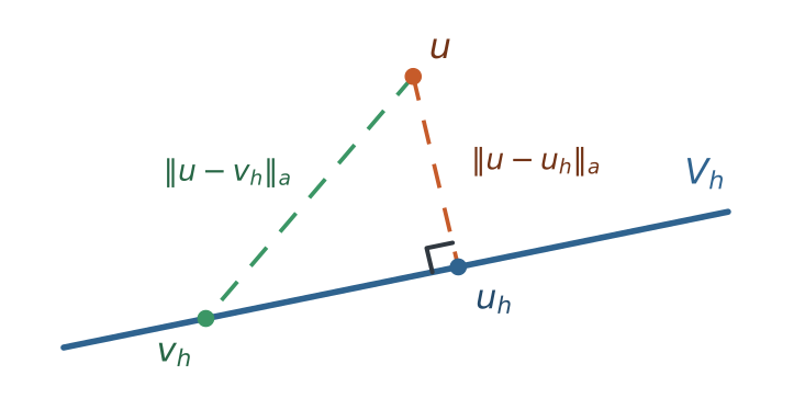
The geometric picture is a point \(u\) outside a line or plane representing \(V_h\). The closest point is measured using the selected norm. For the energy inner product, Galerkin orthogonality makes \(u_h\) the orthogonal projection of \(u\) onto \(V_h\), as illustrated in Figure 7.1.
Example 7.2 (Best approximation depends on the norm) Let \(V=\R^2\), \(V_h=\operatorname{span}\{(1,1)\}\), and \(\bu=(1,0)\). Define
\[ a(\bx,\bm{y})=4x_1y_1+x_2y_2, \qquad \ell(\bm{y})=4y_1, \qquad \norm{\bx}_a=\sqrt{4x_1^2+x_2^2}. \]
The vector \(\bu\) solves the continuous problem because \(a(\bu,\bm{y})=\ell(\bm{y})\) for every \(\bm{y}\in\R^2\). The Galerkin problem restricts the trial and test vectors to \(V_h\).
Every vector in \(V_h\) has the form \(\bv_h=t(1,1)\). The energy-norm error is
\[ \norm{\bu-\bv_h}_a^2 = 4(1-t)^2+t^2. \]
Differentiating this quadratic function of \(t\) gives \(-8(1-t)+2t=0\), so its minimum occurs at \(t=4/5\). Therefore
\[ \bu_h=\left(\frac45,\frac45\right). \]
The same result follows from the Galerkin condition \(a(\bu-\bu_h,(1,1))=0\). In contrast, the closest point in the Euclidean norm is \(\tfrac12(1,1)\). The discrete space is unchanged, but changing the norm changes which point in that space is the best approximation.
7.4 Céa’s lemma
Galerkin orthogonality relates the error to the discrete space, but it does not yet say how large the error is. The next result shows that the finite element error in the \(V\) norm is controlled by Equation 7.13, multiplied by a constant that depends only on the continuity and coercivity constants.
Theorem 7.1 (Céa’s lemma) Let \(V\) be a real Hilbert space with norm \(\norm{\cdot}_V\), let \(a:V\times V\to\R\) be a bilinear form that is continuous with constant \(M\) and coercive with constant \(\alpha\), and let \(\ell\in V^*\). Let \(V_h\subset V\) be a finite-dimensional subspace. If \(u\in V\) satisfies \(a(u,v)=\ell(v)\) for all \(v\in V\), and \(u_h\in V_h\) satisfies \(a(u_h,v_h)=\ell(v_h)\) for all \(v_h\in V_h\), then
\[ \norm{u-u_h}_V \leq \frac{M}{\alpha} \inf_{v_h\in V_h}\norm{u-v_h}_V. \tag{7.15}\]
Proof. The Lax–Milgram theorem Theorem 2.4 gives unique solutions \(u\) and \(u_h\), and they satisfy Galerkin orthogonality Equation 7.10 with \(V\) and \(V_h\) in place of \(\Vzero\) and \(\Vhzero\). Let \(v_h\in V_h\) be arbitrary. Applying the abstract version of the coercivity relation Equation 7.4, with \(\norm{\cdot}_V\) in place of \(\norm{\cdot}_{H^1(\Om)}\), to the error gives
\[ \alpha\norm{u-u_h}_V^2 \leq a(u-u_h,u-u_h). \]
Use \(u-u_h=(u-v_h)+(v_h-u_h)\) in the second argument:
\[ a(u-u_h,u-u_h) = a(u-u_h,u-v_h)+a(u-u_h,v_h-u_h). \]
The last term is zero by Galerkin orthogonality because \(v_h-u_h\in V_h\). Applying the corresponding abstract version of the continuity relation Equation 7.3 to the remaining term gives
\[ \alpha\norm{u-u_h}_V^2 \leq M\norm{u-u_h}_V\norm{u-v_h}_V . \]
If \(u-u_h=0\), there is nothing to prove. Otherwise, divide by \(\alpha\norm{u-u_h}_V\). The resulting inequality holds for every \(v_h\in V_h\), so it also holds for the infimum over \(V_h\). \(\square\)
Céa’s lemma therefore compares the computed error with the best-approximation error Equation 7.13. It separates the error analysis into two independent questions (Süli 2012, 40–42; Arnold 2018, 58–59):
- a stability question, answered by the ratio \(M/\alpha\); and
- an approximation question: how well can functions in the finite element space approximate the exact solution?
A method satisfying Equation 7.15 is called quasi-optimal: its error is at most a fixed multiple of the smallest error attainable in \(V_h\). The factor \(M/\alpha\) does not depend on \(h\) or on \(p\).
For the diffusion problem in the \(H^1(\Om)\) norm, the constants collected in Equation 7.5 give \(M/\alpha=(k_1/k_0)(1+C_P^2)\). The ratio \(k_1/k_0\) is the contrast of the material coefficient. For a body made of materials whose conductivities differ by several orders of magnitude, the \(H^1\) bound becomes pessimistic. When the form is symmetric, the next result shows that the constant in the energy norm is exactly one. The contrast reappears only when an energy-norm estimate is converted into an \(H^1\)-norm estimate using Equation 7.9.
Corollary 7.1 (Best approximation in the energy norm) If, in addition to the hypotheses of Theorem 7.1, the bilinear form \(a\) is symmetric, then
\[ \norm{u-u_h}_a = \min_{v_h\in V_h}\norm{u-v_h}_a . \tag{7.16}\]
Proof. Let \(v_h\in V_h\) be arbitrary. Since \(u_h-v_h\in V_h\), Galerkin orthogonality gives
\[ a(u-u_h,u_h-v_h)=0. \]
Decompose the error associated with \(v_h\) as
\[ u-v_h=(u-u_h)+(u_h-v_h). \]
Because \(a\) is symmetric, it is the inner product associated with \(\norm{\cdot}_a\). Expanding the squared energy norm and using the orthogonality relation therefore gives
\[ \begin{aligned} \norm{u-v_h}_a^2 &=a(u-v_h,u-v_h)\\ &=\norm{u-u_h}_a^2 +2a(u-u_h,u_h-v_h) +\norm{u_h-v_h}_a^2\\ &=\norm{u-u_h}_a^2+\norm{u_h-v_h}_a^2. \end{aligned} \]
The last term is nonnegative. Hence \(\norm{u-u_h}_a\leq\norm{u-v_h}_a\) for every \(v_h\in V_h\). Choosing \(v_h=u_h\) gives equality, so \(u_h\) attains the minimum in Equation 7.14. \(\square\)
In the energy norm, the finite element solution is therefore the best approximation available in the discrete space, with constant one. The error estimates of the next sections bound the right-hand side of Equation 7.16 by choosing one convenient function \(v_h\): the finite element interpolant of \(u\).
Exercise 7.3 (Using Céa’s lemma)
- For the diffusion problem, derive the ratio \(M/\alpha\) in Equation 7.5 from Equation 7.3 and Equation 7.4.
- Use Equation 7.9 and Equation 7.16 to derive a bound of the form \(\norm{u-u_h}_{H^1(\Om)}\leq C\inf_{v_h\in\Vhzero}\norm{u-v_h}_{H^1(\Om)}\). Compare your constant with \(M/\alpha\) in Equation 7.5.
- Let \(\Vh^{\mathrm{dc}}\) be the space of functions that are linear on each element of a triangular mesh but may be discontinuous across element edges. Explain why \(\Vh^{\mathrm{dc}}\not\subset H^1(\Om)\), and identify the step of the derivation of Equation 7.10 that fails if this space is used in 3.
7.5 Interpolation estimates
Céa’s lemma reduces the error analysis to a question about approximation: how small can \(\norm{u-v_h}\) be for some \(v_h\) in the finite element space? It is not necessary to find the best approximation. Any explicit choice of \(v_h\) gives an upper bound. The natural choice is the function in the finite element space that has the same degrees of freedom as \(u\).
7.5.1 The finite element interpolant
Definition 7.2 (Finite element interpolant) Let \(\Vh\) be a Lagrange finite element space with global nodes \(\bx_1,\ldots,\bx_{N_n}\) and nodal basis \(\phi_1,\ldots,\phi_{N_n}\). For a function \(u\) continuous on \(\overline\Om\), the finite element interpolant is
\[ \Ih u = \sum_{i=1}^{N_n}u(\bx_i)\,\phi_i . \tag{7.17}\]
The calligraphic symbol \(\Ih\) denotes the interpolation operator and distinguishes it from the connectivity map \(I^e\). For linear elements, the nodes are the mesh vertices. For higher-degree Lagrange elements they also include additional nodes, such as the element midpoints of the quadratic interval in Chapter 5 and the edge midpoints of the \(P_2\) triangle in Chapter 6.
The interpolant can also be built element by element. In the terminology of Definition 5.1, the local interpolant on \(\mathcal K_e\) is
\[ \Ie w = \sum_{a}N_a(w)\,\phi_a^e , \]
where \(N_a\) are the local degrees of freedom. For a Lagrange element, \(N_a(w)=w(\bx_a^e)\). The local-global relation Equation 6.17 and the nodal property give
\[ (\Ih u)|_{\mathcal K_e} = \Ie\bigl(u|_{\mathcal K_e}\bigr). \]
Figure 7.2 makes this construction visible. On \(\Om=(0,1)^2\), consider the positive function
\[ u(x_1,x_2)=1+x_1(1-x_1)+x_2(1-x_2). \]
Its values at the vertices of the coarse triangular mesh determine the piecewise-planar \(P_1\) interpolant. The exact function, interpolant, and error are evaluated at finer plotting points to display the surfaces clearly. These additional points are not finite element nodes and do not change \(\Ih u\).
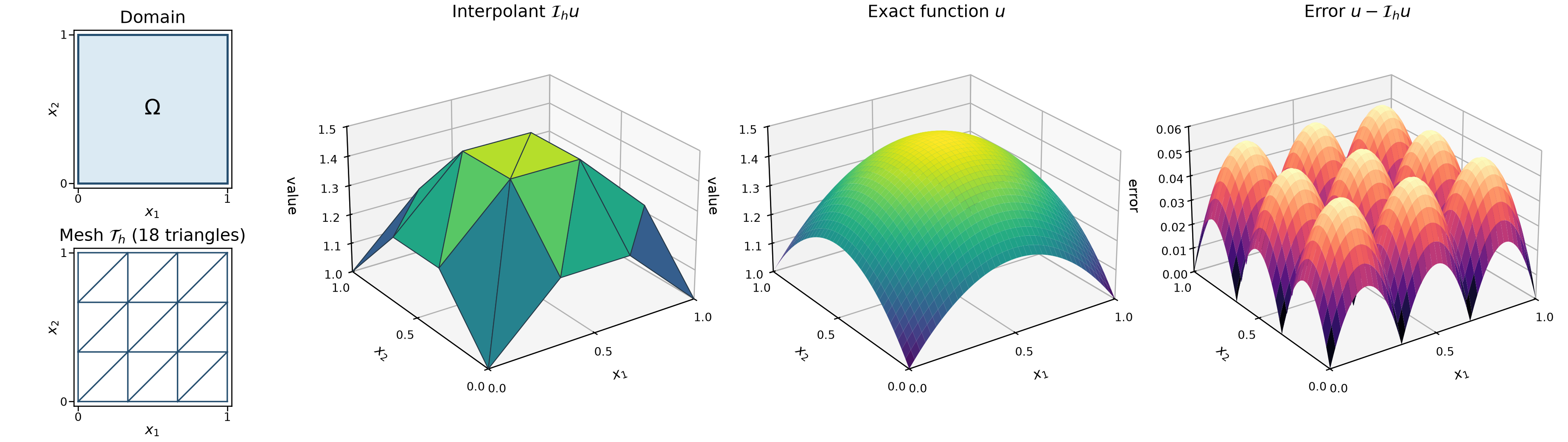
The error is nonnegative for this particular concave function. Moreover, the Hessian of \(u\) is the constant matrix \(-2\bI\), and all triangles in this uniform mesh are congruent. Consequently, the error has the same shape and maximum value on every triangle, up to translation and reflection. Neither the sign nor this repeated error pattern holds for a general function on a general mesh.
Now halve the grid spacing in both coordinate directions. The resulting mesh has \(72\) triangles, compared with \(18\) triangles in Figure 7.2. The refined interpolant in Figure 7.3 follows the exact surface more closely. Both figures use the same vertical scales, including the scale of the error plot.
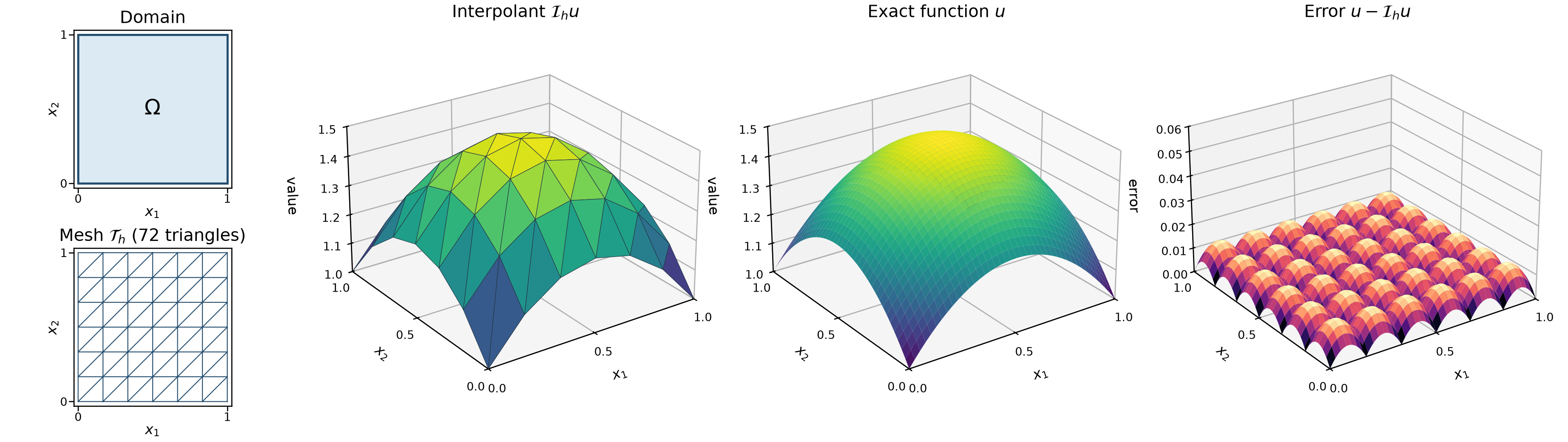
For this quadratic function, the maximum error decreases from \(1/18\) on the coarse mesh to \(1/72\) on the refined mesh. Thus halving the grid spacing reduces the maximum error by a factor of four. This example displays the \(h^2\) behavior of the error in the function values that will be established later in the chapter.
Three properties of the interpolant will be used repeatedly.
- Locality. The restriction of \(\Ih u\) to \(\mathcal K_e\) depends only on the values of \(u\) at the nodes of \(\mathcal K_e\).
- Polynomial reproduction. If \(u|_{\mathcal K_e}\) belongs to the local finite element space, then \(\Ie u=u\) on \(\mathcal K_e\). This does not mean that a degree-\(p\) element reproduces polynomials of arbitrary degree. For an affine Lagrange simplex, the local space is \(\mathbb P_p(\mathcal K_e)\), so every polynomial of total degree at most \(p\) is reproduced exactly. For a tensor-product element, the corresponding statement uses its local \(\mathbb Q_p\) space. On a nonaffine isoparametric element, the local space is defined through the pullback from the reference element and need not consist of polynomials in the physical coordinates. This property generalizes the affine reproduction in Exercise 5.3 and Exercise 6.3.
- Boundary values. If \(u=0\) on \(\Gam_D\) and the mesh resolves \(\Gam_D\), then every node on \(\Gam_D\) has zero value. On each facet contained in \(\Gam_D\), the restriction of \(\Ih u\) is determined by the nodal values on that facet, so \(\Ih u=0\) on \(\Gam_D\) and \(\Ih u\in\Vhzero\).
The interpolant requires point values. For \(d\leq3\) and a bounded Lipschitz domain, every function in \(H^2(\Om)\) has a continuous representative on \(\overline\Om\) (Arnold 2018, 59, 65). In one dimension, every function in \(H^1(0,L)\) is already continuous. In two and three dimensions, a general function in \(H^1(\Om)\) need not be continuous, so the nodal interpolant is not defined for every function in \(\Vzero\). This is why the multidimensional estimates below assume at least \(H^2\) regularity.
7.5.2 Linear interpolation in one dimension
The one-dimensional case shows how an interpolation estimate is obtained. For \(\mathcal K_e=(x_e,x_{e+1})\) and a function \(u\) continuous on \(\overline{\mathcal K}_e\), the linear interpolant is
\[ \Ie u = u(x_e)\,\phi_1^e+u(x_{e+1})\,\phi_2^e , \]
with the local shape functions Equation 5.17.
Figure 7.4 shows the same construction for \(u(x)=1+x(1-x)\) on a uniform mesh of four linear elements. Its five nodes are
\[ x_1=0,\qquad x_2=\frac14,\qquad x_3=\frac12,\qquad x_4=\frac34,\qquad x_5=1. \]
The interpolant agrees with \(u\) at every node and is linear between adjacent nodes. As in Figure 7.2, the finer plotting points only reveal the shapes of the exact function and the error; they are not additional degrees of freedom.
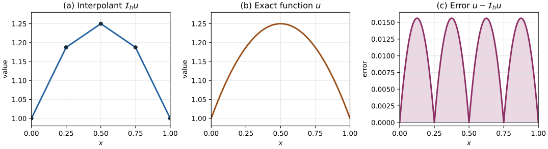
On an element \(\mathcal K_e=[x_e,x_{e+1}]\), direct calculation gives
\[ u(x)-\Ie u(x) = (x-x_e)(x_{e+1}-x). \]
Because every element has length \(h=1/4\), this error has the same shape on every element and reaches the same maximum, \(h^2/4=1/64\), at each element midpoint. This repeated pattern results from combining a uniform mesh with a quadratic function having constant second derivative.
Refine the one-dimensional mesh by dividing every element in two. The refined mesh has eight linear elements and nine nodes, \(x_i=(i-1)/8\) for \(i=1,\ldots,9\). The plots in Figure 7.5 use the same vertical scales as Figure 7.4.
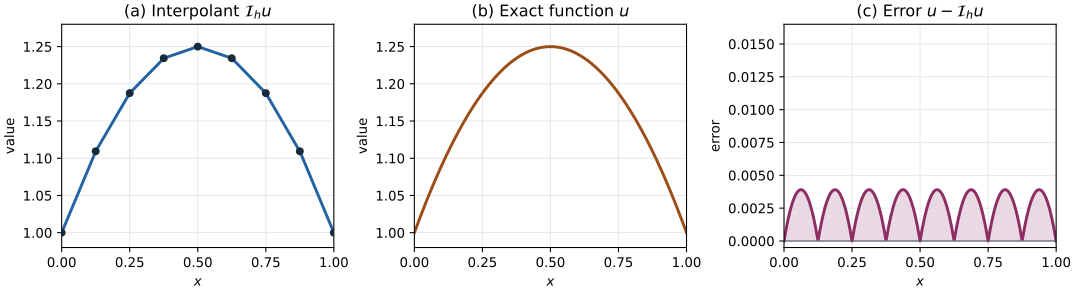
On the refined mesh, \(h=1/8\), so the maximum error is \(h^2/4=1/256\). Halving the element length has again reduced the maximum error by a factor of four.
Theorem 7.2 (Linear interpolation on an interval) Let \(u\in H^2(\mathcal K_e)\). Then
\[ \norm{(u-\Ie u)'}_{L^2(\mathcal K_e)} \leq h_e\norm{u''}_{L^2(\mathcal K_e)}, \qquad \norm{u-\Ie u}_{L^2(\mathcal K_e)} \leq h_e^2\norm{u''}_{L^2(\mathcal K_e)} . \tag{7.18}\]
If \(u\in H^1(0,L)\) and \(u|_{\mathcal K_e}\in H^2(\mathcal K_e)\) for every element, then
\[ \seminorm{u-\Ih u}_{H^1(0,L)}^2 \leq \sum_{e=1}^{N}h_e^2\norm{u''}_{L^2(\mathcal K_e)}^2, \qquad \norm{u-\Ih u}_{L^2(0,L)}^2 \leq \sum_{e=1}^{N}h_e^4\norm{u''}_{L^2(\mathcal K_e)}^2 . \tag{7.19}\]
Proof. Let \(w=u-\Ie u\) on \(\mathcal K_e\). Since \(\Ie u\) is linear, its second derivative is zero. Hence
\[ w''=u'' \qquad\text{on }\mathcal K_e. \]
Moreover, \(u\in H^2(\mathcal K_e)\) implies \(u'\in H^1(\mathcal K_e)\). In one dimension, \(H^1\) functions have continuous representatives. Thus \(u'\) and \(w'\) may be taken to be continuous, \(w\) is continuously differentiable, and the classical fundamental theorem of calculus and Rolle’s theorem can be used.
By the definition of the nodal interpolant,
\[ (\Ie u)(x_e)=u(x_e), \qquad (\Ie u)(x_{e+1})=u(x_{e+1}). \]
Therefore \(w(x_e)=w(x_{e+1})=0\). Rolle’s theorem then gives a point \(x_\ast\in(x_e,x_{e+1})\) such that \(w'(x_\ast)=0\). For any \(y\in\mathcal K_e\), the fundamental theorem of calculus gives
\[ w'(y) = \int_{x_\ast}^{y}w''(t)\,\dd t . \]
Applying the Cauchy–Schwarz inequality on the interval with endpoints \(x_\ast\) and \(y\) gives
\[ |w'(y)|^2 \leq |y-x_\ast|\int_{\min\{x_\ast,y\}}^{\max\{x_\ast,y\}}|w''(t)|^2\,\dd t \leq h_e\norm{w''}_{L^2(\mathcal K_e)}^2 . \]
This pointwise bound holds for every \(y\) in an interval of length \(h_e\). Integrating it with respect to \(y\) therefore gives
\[ \norm{w'}_{L^2(\mathcal K_e)}^2 \leq h_e^2\norm{w''}_{L^2(\mathcal K_e)}^2 = h_e^2\norm{u''}_{L^2(\mathcal K_e)}^2. \]
Taking square roots proves the first local estimate. To estimate \(w\) itself, use \(w(x_e)=0\) and write
\[ w(y)=\int_{x_e}^{y}w'(t)\,\dd t. \]
Another application of Cauchy–Schwarz gives
\[ |w(y)|^2 \leq (y-x_e)\int_{x_e}^{y}|w'(t)|^2\,\dd t \leq h_e\norm{w'}_{L^2(\mathcal K_e)}^2. \]
Integrating over \(y\in\mathcal K_e\) and taking square roots yields
\[ \norm{w}_{L^2(\mathcal K_e)} \leq h_e\norm{w'}_{L^2(\mathcal K_e)}. \]
Combining this inequality with the first local estimate proves the second. Finally, the elements have disjoint interiors, so the squared global norms are the sums of the squared element norms. Summing the local estimates gives Equation 7.19. \(\square\)
The proof follows Larson and Bengzon (2010, 5–7). Sharper constants are available: a Fourier-series argument replaces \(h_e\) by \(h_e/\pi\) in both estimates (Süli 2012, 46–47). The powers of \(h_e\) are what matter for convergence rates. Using \(h_e\leq h\) in Equation 7.19 gives
\[ \seminorm{u-\Ih u}_{H^1(0,L)} \leq h\norm{u''}_{L^2(0,L)}, \qquad \norm{u-\Ih u}_{L^2(0,L)} \leq h^2\norm{u''}_{L^2(0,L)} \]
when \(u\in H^2(0,L)\). The elementwise form is more informative: it shows that small elements are most useful where \(|u''|\) is large, which is the idea behind the adaptive meshes of Chapter 8.
The one-dimensional bar has an additional property that explains the exact nodal values observed in Chapter 5.
Example 7.3 (When the finite element solution equals the interpolant) Consider the bar problem Equation 5.27 with linear elements, and assume that \(AE\) is constant on each element, with value \((AE)_e\) on \(\mathcal K_e\). The load \(f\in L^2(0,L)\) and the end force \(\overline P\) are arbitrary. The exact solution \(u\) belongs to \(H^1(0,L)\) and is therefore continuous, so \(\Ih u\) is defined; it belongs to \(\Vhzero\) because \(u(0)=0\).
Let \(v_h\in\Vhzero\). Its derivative is a constant \(v_h'|_e\) on each element, so
\[ a(u-\Ih u,v_h) = \sum_{e=1}^{N}(AE)_e\,v_h'|_e \int_{x_e}^{x_{e+1}}(u-\Ih u)'\,\dd x = \sum_{e=1}^{N}(AE)_e\,v_h'|_e \Bigl[(u-\Ih u)(x)\Bigr]_{x_e}^{x_{e+1}} =0, \]
because the interpolation error vanishes at every node. Galerkin orthogonality Equation 7.10 gives \(a(u-u_h,v_h)=0\) as well. Subtracting,
\[ a(u_h-\Ih u,v_h)=0 \qquad\forall v_h\in\Vhzero . \]
Choosing \(v_h=u_h-\Ih u\) and using coercivity gives \(u_h=\Ih u\). The finite element solution is the interpolant of the exact solution, so its nodal values are exact and its whole error is interpolation error.
For the problem of Example 5.5, with \(L=AE=f_0=1\) and \(u(x)=x-x^2/2\), the error on an element of length \(h\) is therefore the interpolation error of a quadratic with \(u''=-1\). With \(s=x-x_e\),
\[ e(x)=\frac{s(h-s)}{2}, \qquad e'(x)=\frac{h-2s}{2}, \qquad 0\leq s\leq h . \]
Direct integration over one element gives \(\int_0^h e^2\,\dd s=h^5/120\) and \(\int_0^h(e')^2\,\dd s=h^3/12\). Summing over \(N=1/h\) elements,
\[ \max_{x}|e(x)|=\frac{h^2}{8}, \qquad \norm{e}_{L^2(0,1)}=\frac{h^2}{\sqrt{120}}, \qquad \norm{e}_a=\seminorm{e}_{H^1(0,1)}=\frac{h}{\sqrt{12}} . \tag{7.20}\]
The maximum error \(h^2/8\) is the value reported in the legend of Figure 5.11. The displacement errors decrease like \(h^2\), whereas the strain error decreases only like \(h\). The estimates of Theorem 7.2, with \(\norm{u''}_{L^2(0,1)}=1\), give the upper bounds \(h^2\) and \(h\), so they predict the correct powers of \(h\) with conservative constants.
Exact nodal values are a special property of this one-dimensional problem with elementwise-constant \(AE\). They do not hold in general in two or three dimensions. A convergence study should therefore never measure the error only at the nodes.
Exercise 7.4 (A pointwise interpolation estimate) Let \(u\in C^2(\overline{\mathcal K}_e)\) and \(w=u-\Ie u\).
- For a fixed \(y\) in the interior of \(\mathcal K_e\), define \[ \psi(x)=w(x)-w(y)\, \frac{(x-x_e)(x-x_{e+1})}{(y-x_e)(y-x_{e+1})}. \] Show that \(\psi\) vanishes at three points of \(\overline{\mathcal K}_e\), and use Rolle’s theorem twice to prove that \(w(y)=\tfrac12u''(\bar x)(y-x_e)(y-x_{e+1})\) for some \(\bar x\in\mathcal K_e\).
- Deduce \(\max_{\overline{\mathcal K}_e}|w|\leq \tfrac18h_e^2\max_{\overline{\mathcal K}_e}|u''|\).
- Show that the bound in Part 2 is attained for \(u(x)=x-x^2/2\), and compare it with the exact error expressions in 2.
7.5.3 Mesh size and shape regularity
In two and three dimensions, the size of an element is not the only geometric quantity that affects interpolation. A long thin triangle and an equilateral triangle can have the same diameter but very different interpolation properties. We therefore measure the shape of each element.
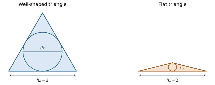
Definition 7.3 (Shape-regular family of meshes) For an element \(\mathcal K_e\), let \(h_e=\operatorname{diam}(\mathcal K_e)\) as in Equation 6.2, and let \(\rho_e\) be the diameter of the largest ball contained in \(\mathcal K_e\). The ratio \(h_e/\rho_e\geq1\) is the shape parameter of the element. A family of meshes \(\{\Th\}_{h>0}\) is shape regular if there is a constant \(\sigma\geq1\) such that
\[ \frac{h_e}{\rho_e}\leq\sigma \qquad \text{for every element }\mathcal K_e\in\Th\text{ and every mesh in the family.} \tag{7.21}\]
The definition concerns a family of meshes rather than a single mesh because convergence is a statement about a sequence of refinements. Every single mesh has some finite bound \(\sigma\); shape regularity requires that repeated refinement does not make the elements progressively flatter. For triangles, a uniform bound on \(h_e/\rho_e\) is equivalent to a uniform positive lower bound on the interior angles, and interpolation constants for linear triangles grow as the smallest angle decreases (Larson and Bengzon 2010, 52). In one dimension, \(\rho_e=h_e\) and every family of meshes is shape regular.
For general degree, we use the \(H^s\) seminorm of an integer order \(s\geq1\),
\[ \seminorm{v}_{H^s(\Om)}^2 = \sum_{|\alpha|=s}\norm{D^\alpha v}_{L^2(\Om)}^2, \tag{7.22}\]
which extends Equation 2.53 with the multi-index notation of Definition 2.18. The elementwise seminorm \(\seminorm{v}_{H^s(\mathcal K_e)}\) is defined in the same way with \(\Om\) replaced by \(\mathcal K_e\).
The role of \(\rho_e\) becomes clear when an interpolation estimate is transferred from the reference element to a physical element. The details of this step are included in the proof below because they explain why a bound on element diameters alone is insufficient.
Theorem 7.3 (Interpolation estimate for Lagrange elements) Let \(d\leq3\), and let \(\{\Th\}\) be a shape-regular family of conforming affine simplicial meshes of a polygonal or polyhedral domain \(\Om\), with shape bound \(\sigma\). Let \(\Vh\) be the continuous Lagrange space of degree \(p\geq1\), and let \(s\) be an integer with \(2\leq s\leq p+1\). There is a constant \(C_I\), depending only on \(d\), \(p\), \(s\), and \(\sigma\), such that for every \(u\in H^s(\Om)\) and every element \(\mathcal K_e\in\Th\),
\[ \norm{u-\Ie u}_{L^2(\mathcal K_e)} \leq C_I\,h_e^s\seminorm{u}_{H^s(\mathcal K_e)}, \qquad \seminorm{u-\Ie u}_{H^1(\mathcal K_e)} \leq C_I\,h_e^{s-1}\seminorm{u}_{H^s(\mathcal K_e)} . \tag{7.23}\]
Consequently,
\[ \norm{u-\Ih u}_{L^2(\Om)} \leq C_I\,h^s\seminorm{u}_{H^s(\Om)}, \qquad \seminorm{u-\Ih u}_{H^1(\Om)} \leq C_I\,h^{s-1}\seminorm{u}_{H^s(\Om)} . \tag{7.24}\]
Proof. Let \(\widehat{\mathcal K}\) be the fixed reference simplex, and let \(\Iref\) denote its degree-\(p\) nodal interpolation operator. The Bramble–Hilbert lemma, together with the fact that \(\Iref\) reproduces every polynomial in \(\mathbb P_p(\widehat{\mathcal K})\), gives
\[ \norm{\widehat{u}-\Iref\widehat{u}}_{L^2(\widehat{\mathcal K})} \leq C_{\mathrm{ref}}\seminorm{\widehat{u}}_{H^s(\widehat{\mathcal K})}, \qquad \seminorm{\widehat{u}-\Iref\widehat{u}}_{H^1(\widehat{\mathcal K})} \leq C_{\mathrm{ref}}\seminorm{\widehat{u}}_{H^s(\widehat{\mathcal K})}, \tag{7.25}\]
for \(2\leq s\leq p+1\). The constant \(C_{\mathrm{ref}}\) depends on the fixed reference element, \(p\), and \(s\), but not on a physical element or its size. For \(d\leq3\) and \(s\geq2\), the functions have well-defined nodal values, so the nodal interpolants in Equation 7.25 are defined.
Let the affine map from the reference element to \(\mathcal K_e\) be
\[ \bx=\bx^e(\widehat{\bx})=\bx_1^e+\bm J_e\widehat{\bx}, \qquad \widehat{u}=u\circ \bx^e . \]
Because the physical interpolation nodes are the images of the reference nodes, interpolation commutes with this map:
\[ (\Ie u)\circ \bx^e=\Iref\widehat{u} . \tag{7.26}\]
For any \(v\) on \(\mathcal K_e\), let \(\widehat{v}=v\circ \bx^e\). The change of variables formula and the gradient transformation of Equation 6.27 give
\[ \norm{v}_{L^2(\mathcal K_e)} = |\det\bm J_e|^{1/2} \norm{\widehat{v}}_{L^2(\widehat{\mathcal K})}, \qquad \seminorm{v}_{H^1(\mathcal K_e)} \leq C|\det\bm J_e|^{1/2}\norm{\bm J_e^{-1}} \seminorm{\widehat{v}}_{H^1(\widehat{\mathcal K})}. \tag{7.27}\]
Applying the chain rule \(s\) times to \(\widehat{u}=u\circ \bx^e\) gives the corresponding bound for its derivatives,
\[ \seminorm{\widehat{u}}_{H^s(\widehat{\mathcal K})} \leq C|\det\bm J_e|^{-1/2}\norm{\bm J_e}^{s} \seminorm{u}_{H^s(\mathcal K_e)} . \tag{7.28}\]
The determinant factors cancel when Equation 7.25–Equation 7.28 are combined with \(v=u-\Ie u\). The geometry of an affine simplex gives
\[ \norm{\bm J_e}\leq C h_e, \qquad \norm{\bm J_e^{-1}}\leq \frac{C}{\rho_e}. \tag{7.29}\]
We therefore obtain the estimates before imposing shape regularity:
\[ \norm{u-\Ie u}_{L^2(\mathcal K_e)} \leq Ch_e^s\seminorm{u}_{H^s(\mathcal K_e)}, \qquad \seminorm{u-\Ie u}_{H^1(\mathcal K_e)} \leq C\frac{h_e}{\rho_e}h_e^{s-1} \seminorm{u}_{H^s(\mathcal K_e)} . \tag{7.30}\]
The second estimate shows explicitly where element shape enters. Shape regularity replaces \(h_e/\rho_e\) by the mesh-independent bound \(\sigma\), which proves Equation 7.23.
It remains to pass from the element estimates to the whole domain. Since the element interiors are disjoint and \(h_e\leq h\),
\[ \begin{aligned} \norm{u-\Ih u}_{L^2(\Om)}^2 &= \sum_{\mathcal K_e\in\Th} \norm{u-\Ie u}_{L^2(\mathcal K_e)}^2 \\ &\leq C_I^2\sum_{\mathcal K_e\in\Th} h_e^{2s}\seminorm{u}_{H^s(\mathcal K_e)}^2 \\ &\leq C_I^2h^{2s}\seminorm{u}_{H^s(\Om)}^2, \end{aligned} \]
and, in the same way,
\[ \seminorm{u-\Ih u}_{H^1(\Om)}^2 \leq C_I^2h^{2(s-1)}\seminorm{u}_{H^s(\Om)}^2. \]
Taking square roots gives Equation 7.24. The same argument applies for every degree \(p\): polynomial reproduction on the reference element allows the Bramble–Hilbert estimate through derivative order \(s\leq p+1\), and the affine scaling is unchanged. \(\square\)
Arnold gives a constructive proof of the Bramble–Hilbert lemma and then uses it in this scaling argument (Arnold 2018, 61–65, Theorems 4.2–4.6). A more general treatment appears in (Süli 2012, 75–83, Lemma 12, Theorem 9, and Equations (3.4)–(3.6)).
Four features of the theorem deserve emphasis.
First, the general estimate guarantees at most order \(p\) in the \(H^1\) seminorm and order \(p+1\) in \(L^2\), even for smoother \(u\). Particular solutions can be represented exactly or exhibit faster convergence; an upper error bound is not a lower bound on the error. The interpolant reproduces polynomials of degree \(p\) but not of degree \(p+1\), and the upper limit \(s\leq p+1\) records this fact.
Second, the estimate guarantees order \(s-1\) in the \(H^1\) seminorm when only \(s\) square-integrable derivatives are assumed. Increasing \(p\) therefore improves the rate only when the exact solution has the corresponding smoothness.
Third, the lower limit \(s\geq2\) ensures that point values exist. Estimates for less regular functions require a different quasi-interpolation operator; such operators are used in the a posteriori analysis of Chapter 8 (Arnold 2018, 67–68).
Fourth, the theorem is stated for affine simplicial elements. For quadrilateral and hexahedral elements, the reference space \(\mathbb Q_p\) contains \(\mathbb P_p\), and estimates of the same form hold on meshes of parallelograms and parallelepipeds. Nonaffine isoparametric elements require additional conditions on the geometry map, which we do not develop.
Exercise 7.5 (A triangle with an angle near \(180^\circ\)) For \(0<\epsilon\leq1\), consider the triangle \(\mathcal K_\epsilon\) with vertices \((-1,0)\), \((1,0)\), and \((0,\epsilon)\), and let \(u(x,y)=x^2\).
- Compute \(h_e\) and \(\rho_e\) for \(\mathcal K_\epsilon\), using the fact that the inscribed circle has radius equal to the area divided by the semiperimeter. Show that \(h_e/\rho_e\) grows like \(1/\epsilon\) as \(\epsilon\to0\).
- Show that the linear interpolant of \(u\) on \(\mathcal K_\epsilon\) is \(\Ie u=1-y/\epsilon\).
- Compute \(\seminorm{u}_{H^2(\mathcal K_\epsilon)}^2\) and \(\seminorm{u-\Ie u}_{H^1(\mathcal K_\epsilon)}^2\).
- Explain why no estimate of the form \(\seminorm{u-\Ie u}_{H^1(\mathcal K_e)}\leq
Ch_e\seminorm{u}_{H^2(\mathcal K_e)}\) can hold with a constant \(C\) independent of \(\epsilon\). Relate the result to the shape parameter in
7.6 Convergence in the energy and \(H^1\) norms
We can now combine the best-approximation property with the interpolation estimate.
Theorem 7.4 (Energy-norm and \(H^1\)-norm convergence) Assume the diffusion problem and finite element spaces defined by Equation 7.1 and 3, with a shape-regular family of affine simplicial meshes and Lagrange elements of degree \(p\geq1\). If \(u\in H^s(\Om)\) for an integer \(s\) with \(2\leq s\leq p+1\), then
\[ \norm{u-u_h}_a \leq C_I\sqrt{k_1}\;h^{s-1}\seminorm{u}_{H^s(\Om)} \tag{7.31}\]
and
\[ \norm{u-u_h}_{H^1(\Om)} \leq C_I\sqrt{\frac{k_1(1+C_P^2)}{k_0}}\;h^{s-1}\seminorm{u}_{H^s(\Om)}, \tag{7.32}\]
where \(C_I\) is the constant of Theorem 7.3.
Proof. Since \(u\in H^s(\Om)\) with \(s\geq2\), the interpolant \(\Ih u\) is defined, and it belongs to \(\Vhzero\) by the boundary-value property of Section 7.5. The diffusion form is symmetric, so Corollary 7.1 applies with \(v_h=\Ih u\). The upper bound in Equation 7.8 and Equation 7.24 then give
\[ \norm{u-u_h}_a \leq \norm{u-\Ih u}_a \leq \sqrt{k_1}\,\seminorm{u-\Ih u}_{H^1(\Om)} \leq C_I\sqrt{k_1}\,h^{s-1}\seminorm{u}_{H^s(\Om)} . \]
For the \(H^1\) norm, Corollary 2.2 and the lower bound in Equation 7.8 give, for every \(v\in\Vzero\),
\[ \norm{v}_{H^1(\Om)} \leq \sqrt{1+C_P^2}\,\seminorm{v}_{H^1(\Om)} \leq \sqrt{\frac{1+C_P^2}{k_0}}\,\norm{v}_a . \]
Applying this inequality to \(v=u-u_h\) and using Equation 7.31 gives Equation 7.32. \(\square\)
When \(u\) is smooth enough that \(u\in H^{p+1}(\Om)\), the choice \(s=p+1\) gives
\[ \norm{u-u_h}_a=O(h^p), \qquad \norm{u-u_h}_{H^1(\Om)}=O(h^p). \]
Here \(E(h)=O(h^r)\) means that \(E(h)\leq Ch^r\) for a constant \(C\) independent of \(h\). Linear elements therefore converge at first order in the energy norm, and quadratic elements at second order, provided \(u\in H^2(\Om)\) or \(u\in H^3(\Om)\), respectively. The exponent \(r\) in such a bound is called the convergence rate, or order of convergence, in that norm.
The same estimate controls the flux or, in one dimension, the axial force. Because \(k\leq k_1\),
\[ \norm{k\grad u-k\grad u_h}_{L^2(\Om;\R^d)} \leq \sqrt{k_1}\,\norm{u-u_h}_a , \]
so the flux error converges at the same rate as the energy error. For affine linear elements the computed gradient is piecewise constant. The flux is piecewise constant only when \(k\) is also constant on each element. Under the stated regularity assumptions its error is bounded by \(O(h)\), as the strains in Example 5.4 suggest.
Several practical consequences follow from the hypotheses of the theorem.
Mesh size and degrees of freedom. A family of meshes is called quasi-uniform if, in addition to shape regularity, there is a constant \(c>0\) with \(h_e\geq ch\) for every element. On such meshes the number of elements, and hence for fixed \(p\) the number of degrees of freedom \(N_{\mathrm{dof}}\), is proportional to \(h^{-d}\). An energy-norm rate \(h^{p}\) therefore corresponds to \(N_{\mathrm{dof}}^{-p/d}\). In three dimensions, halving \(h\) multiplies the number of unknowns by about eight but reduces the energy error of linear elements by only a factor of about two.
The rate is limited by the smaller of \(p\) and the available regularity. If the solution belongs to \(H^s(\Om)\) but not to \(H^{s+1}(\Om)\), then elements of degree higher than \(s-1\) do not improve the guaranteed rate on quasi-uniform meshes. The smoothness of \(u\) depends on the data and on the geometry. For example, on a polygon with a reentrant corner, the solution of the Laplace problem may fail to belong to \(H^2(\Om)\). In that case the hypotheses needed for the linear-element \(O(h)\) energy-norm estimate are not available, and raising the polynomial degree does not restore that guarantee. Locally refined meshes can resolve such localized loss of regularity more economically than uniform refinement, which is one motivation for Chapter 8.
\(h\)-refinement and \(p\)-refinement. The estimate describes \(h\)-refinement with a fixed degree \(p\): the constant \(C_I\) depends on \(p\). It does not by itself describe the limit \(p\to\infty\) on a fixed mesh, for which a separate approximation theory is needed and is not developed in this book. What the estimate does say is that, on a fixed sequence of meshes, raising \(p\) raises the attainable rate from \(h^{p}\) to \(h^{p+1}\) only when \(u\) has the additional smoothness.
The estimate usually does not supply a numerical error value. The right-hand side contains \(\seminorm{u}_{H^s(\Om)}\), which depends on the unknown solution, and \(C_I\), which is rarely known sharply. An a priori estimate predicts the rate of convergence and the dependence on the mesh and the material, but it does not give a reliable number for the error in a given computation (Süli 2012, 42). That is the purpose of the a posteriori estimates of Chapter 8.
Exercise 7.6 (Predicting convergence rates) Assume the hypotheses of Theorem 7.4.
- Complete a table of the guaranteed energy-norm rate for \(p=1,2,3\) when the largest integer \(s\) with \(u\in H^s(\Om)\) is \(s=2\), \(3\), and \(4\).
- For a two-dimensional quasi-uniform mesh and linear elements, estimate the factor by which the energy error decreases when \(N_{\mathrm{dof}}\) is multiplied by \(16\). Repeat for quadratic elements with \(u\in H^3(\Om)\).
- Explain why the rate for \(p=3\) and \(s=2\) is not better than the rate for \(p=1\) and \(s=2\), and state what information about \(u\) would justify using cubic elements.
7.7 \(L^2\) estimates by duality
The \(L^2\) norm is bounded by the \(H^1\) norm, so Equation 7.32 already implies \(\norm{u-u_h}_{L^2(\Om)}=O(h^{s-1})\). For the bar problem of Chapter 5, the exact expressions in 2 show an \(L^2\) error proportional to \(h^2\) with linear elements, one power of \(h\) faster. The interpolation estimate Equation 7.24 also has one more power of \(h\) in \(L^2\) than in the \(H^1\) seminorm. Céa’s lemma cannot transfer that extra power because it holds in the norm in which \(a\) is coercive. A different argument is needed. It uses an auxiliary problem, called the dual problem, whose solution converts the \(L^2\) error into an energy product to which Galerkin orthogonality applies. The argument is known as the Aubin–Nitsche duality argument.
Recall that the diffusion bilinear form is
\[ a(w,v)=\int_\Om k\grad w\cdot\grad v\,\dx. \]
For a given \(r\in L^2(\Om)\), the dual problem is
\[ \text{find }z\in\Vzero\text{ such that}\qquad a(v,z)=\inner{r}{v}_{L^2(\Om)} \qquad\forall v\in\Vzero . \tag{7.33}\]
The unknown \(z\) appears in the second argument of \(a\). For the symmetric diffusion form this makes no difference. Using the flux convention of Equation 3.6, Equation 7.33 is the variational form of
\[ \begin{aligned} -\divg(k\grad z)&=r &&\text{in }\Om,\\ z&=0 &&\text{on }\Gam_D,\\ k\grad z\cdot\bn&=0 &&\text{on }\Gam_N. \end{aligned} \tag{7.34}\]
For a nonsymmetric form, placing \(z\) in the second argument produces the adjoint problem. Since \(v\mapsto\inner{r}{v}_{L^2(\Om)}\) is a continuous linear functional on \(\Vzero\), the Lax–Milgram theorem gives a unique \(z\).
The duality argument needs more smoothness of \(z\) than the Lax–Milgram theorem provides.
Definition 7.4 (\(H^2\) regularity of the dual problem) The dual problem Equation 7.33 is \(H^2\)-regular if there is a constant \(C_{\mathrm{reg}}\) such that, for every \(r\in L^2(\Om)\), its solution satisfies \(z\in H^2(\Om)\) and
\[ \seminorm{z}_{H^2(\Om)} \leq C_{\mathrm{reg}}\norm{r}_{L^2(\Om)} . \tag{7.35}\]
This is a property of the domain, the coefficient, and the boundary partition, not of the mesh. It holds, for example, for the one-dimensional bar with constant \(AE\) (Exercise 7.7), and for a convex polygonal domain with \(\Gam_D=\partial\Om\) and a constant or smooth coefficient (Arnold 2018, 66). It can fail near reentrant corners, near points where the boundary condition changes type, and across jumps in \(k\). In those cases the duality argument yields less than a full additional power of \(h\).
The proof below has three steps. First, choose the right-hand side of the dual problem to be the finite element error \(e=u-u_h\); this expresses \(\norm{e}_{L^2(\Om)}^2\) as \(a(e,z)\). Second, use Galerkin orthogonality to replace \(z\) by its interpolation error \(z-\Ih z\). Third, use the \(H^2\) regularity of \(z\) to bound this interpolation error by \(Ch\norm{e}_{L^2(\Om)}\). This last factor of \(h\) produces the improved \(L^2\) rate.
Theorem 7.5 (\(L^2\) convergence by duality) Assume the hypotheses of Theorem 7.4, and assume that the dual problem is \(H^2\)-regular. Then
\[ \norm{u-u_h}_{L^2(\Om)} \leq k_1C_IC_{\mathrm{reg}}\;h\;\seminorm{u-u_h}_{H^1(\Om)} , \tag{7.36}\]
and consequently
\[ \norm{u-u_h}_{L^2(\Om)} \leq C_I^2C_{\mathrm{reg}}\,k_1\sqrt{\frac{k_1}{k_0}}\; h^{s}\seminorm{u}_{H^s(\Om)} . \tag{7.37}\]
Here \(C_I\) is a constant for which Equation 7.24 holds both for the given \(s\) and for \(s=2\).
Proof. Let \(e=u-u_h\in\Vzero\) and solve the dual problem with \(r=e\). Taking \(v=e\) in Equation 7.33 gives
\[ \norm{e}_{L^2(\Om)}^2 = \inner{e}{e}_{L^2(\Om)} = a(e,z). \]
The dual solution \(z\) belongs to \(H^2(\Om)\cap\Vzero\), so \(\Ih z\) is defined and lies in \(\Vhzero\). Choose \(v_h=\Ih z\) in Galerkin orthogonality Equation 7.10. This gives
\[ a(e,\Ih z)=0. \]
Therefore, bilinearity in the second argument gives
\[ \norm{e}_{L^2(\Om)}^2 = a(e,z)-a(e,\Ih z) = a(e,z-\Ih z). \]
The coefficient bound \(k\leq k_1\) and the Cauchy–Schwarz inequality give
\[ |a(w,v)| \leq k_1\seminorm{w}_{H^1(\Om)}\seminorm{v}_{H^1(\Om)}. \]
Apply this estimate to \(a(e,z-\Ih z)\), then use the interpolation estimate Equation 7.24 with \(s=2\) and the regularity estimate Equation 7.35 with \(r=e\):
\[ \begin{aligned} \norm{e}_{L^2(\Om)}^2 &=a(e,z-\Ih z)\\ &\leq k_1\seminorm{e}_{H^1(\Om)} \seminorm{z-\Ih z}_{H^1(\Om)}\\ &\leq k_1C_I\,h\seminorm{e}_{H^1(\Om)}\seminorm{z}_{H^2(\Om)}\\ &\leq k_1C_IC_{\mathrm{reg}}\,h\seminorm{e}_{H^1(\Om)} \norm{e}_{L^2(\Om)}. \end{aligned} \]
Dividing by \(\norm{e}_{L^2(\Om)}\), when it is nonzero, gives Equation 7.36. The lower bound in Equation 7.8 and the energy estimate Equation 7.31 give
\[ \seminorm{e}_{H^1(\Om)} \leq \frac{1}{\sqrt{k_0}}\norm{e}_a \leq C_I\sqrt{\frac{k_1}{k_0}}\,h^{s-1} \seminorm{u}_{H^s(\Om)}. \]
Substituting this estimate into Equation 7.36 gives Equation 7.37. \(\square\)
The proof follows Arnold (2018, 66–67). The extra power of \(h\) comes from the interpolation error of the dual solution: Galerkin orthogonality lets us replace \(z\) by \(z-\Ih z\), which is small because \(z\) is smooth. For smooth solutions with \(s=p+1\), the result is
\[ \norm{u-u_h}_{L^2(\Om)}=O(h^{p+1}), \]
one order higher than the energy-norm rate. For linear elements this is the second-order \(L^2\) convergence seen in Chapter 5.
For a solution smooth enough that \(u\in H^{p+1}(\Om)\), the estimates predict the following rates:
| Polynomial degree \(p\) | Energy and \(H^1\) errors | \(L^2\) error |
|---|---|---|
| 1 | \(O(h)\) | \(O(h^2)\) |
| 2 | \(O(h^2)\) | \(O(h^3)\) |
| 3 | \(O(h^3)\) | \(O(h^4)\) |
The \(L^2\) column additionally requires \(H^2\) regularity of the dual problem. If either the exact solution lacks \(H^{p+1}\) regularity or the dual solution lacks \(H^2\) regularity, the corresponding rate is not guaranteed.
The same argument estimates the error in other linear quantities of interest. If \(Q(v)=\inner{w_Q}{v}_{L^2(\Om)}\) for a fixed \(w_Q\in L^2(\Om)\), solving the dual problem with \(r=w_Q\) gives \(Q(u)-Q(u_h)=a(e,z-\Ih z)\) and hence a bound of order \(h\,\seminorm{e}_{H^1(\Om)}\) (Arnold 2018, 66–67). Chapter 8 returns to this goal-oriented use of duality.
Exercise 7.7 (Duality for the axial bar) Let \(AE\) be constant on \((0,L)\) and \(\mathcal V_0=\{v\in H^1(0,L):v(0)=0\}\).
- Show that the dual problem Equation 7.33 is the weak form of \(-AE\,z''=r\) in \((0,L)\) with \(z(0)=0\) and \(AE\,z'(L)=0\).
- Verify that \[ z'(x)=\frac{1}{AE}\int_x^L r(t)\,\dd t, \qquad z(x)=\int_0^x z'(t)\,\dd t \] solves this problem, and prove that \(\seminorm{z}_{H^2(0,L)}= \norm{r}_{L^2(0,L)}/AE\). Thus the dual problem is \(H^2\)-regular with \(C_{\mathrm{reg}}=1/AE\).
- Use Theorem 7.2, which gives \(C_I=1\) in one dimension, and the argument of Theorem 7.5 to prove \(\norm{u-u_h}_{L^2(0,L)}\leq h\,\seminorm{u-u_h}_{H^1(0,L)}\) for linear elements. Note that \(AE\) cancels.
- Check this inequality against the exact values in
7.8 Numerical verification of convergence rates
A convergence estimate is also a test of an implementation. If a code solves a problem with a known smooth solution and the observed rates differ from the predicted rates, then either the hypotheses are not satisfied or the code contains an error. Checking rates is therefore a standard part of code verification.
Suppose an error measure \(E\) has been computed on two meshes with sizes \(h_1\) and \(h_2<h_1\). If \(E(h)\approx Ch^r\) on both meshes, then \(E(h_1)/E(h_2)\approx(h_1/h_2)^r\). The observed convergence rate is therefore defined by
\[ r_{\mathrm{obs}} = \frac{\log\bigl(E(h_1)/E(h_2)\bigr)}{\log(h_1/h_2)} . \tag{7.38}\]
For successive uniform refinements with \(h_2=h_1/2\), this becomes \(r_{\mathrm{obs}}=\log\bigl(E(h)/E(h/2)\bigr)/\log2\). Equivalently, \(r\) is the slope of the error curve on a log–log plot.
A meaningful study requires the following:
- an exact solution, often obtained by the method of manufactured solutions: choose a smooth \(u\), compute the source and boundary data that it satisfies, and solve with those data;
- a sequence of meshes, typically obtained by uniform refinement, that satisfies the hypotheses of the theorem being tested;
- an error computed by integrating \(u-u_h\) and its derivatives with a quadrature rule of sufficiently high order on every element, rather than by sampling at the nodes alone; and
- meshes fine enough to be in the asymptotic range, where Equation 7.38 has stabilized, but not so fine that rounding error in the solve dominates the discretization error.
Example 7.4 (Rates for the uniformly loaded bar) For the problem of Example 5.5, the exact expressions in 2 give the errors on uniform meshes exactly:
| \(N\) | \(h\) | \(\max_x\lvert e\rvert\) | \(\norm{e}_{L^2(0,1)}\) | \(\norm{e}_a\) |
|---|---|---|---|---|
| 2 | \(1/2\) | \(3.125\times10^{-2}\) | \(2.282\times10^{-2}\) | \(1.443\times10^{-1}\) |
| 4 | \(1/4\) | \(7.813\times10^{-3}\) | \(5.705\times10^{-3}\) | \(7.217\times10^{-2}\) |
| 8 | \(1/8\) | \(1.953\times10^{-3}\) | \(1.426\times10^{-3}\) | \(3.608\times10^{-2}\) |
| 16 | \(1/16\) | \(4.883\times10^{-4}\) | \(3.566\times10^{-4}\) | \(1.804\times10^{-2}\) |
Every halving of \(h\) divides the first two errors by four and the energy error by two, so Equation 7.38 gives exactly \(2\), \(2\), and \(1\). These values agree with Theorem 7.4 and Theorem 7.5 for \(p=1\) and \(s=2\); the dual problem is \(H^2\)-regular by Exercise 7.7. The \(H^1\) norm, \(\bigl(\norm{e}_{L^2}^2+\norm{e}_a^2\bigr)^{1/2}\) here, also converges at first order, although on coarse meshes its observed rate is slightly above one because it contains the faster-decaying \(L^2\) part.
The exact solution in this example is quadratic. It belongs to the quadratic finite element space, so quadratic elements reproduce it exactly (Example 5.6) and cannot be used to observe a rate. The next example manufactures a nonpolynomial solution and compares linear and quadratic elements.
Example 7.5 (Manufactured solution with linear and quadratic elements) Choose
\[ u(x)=\sin\frac{\pi x}{2} \qquad\text{on }(0,1). \]
Then \(u(0)=0\), \(u'(1)=0\), and \(-u''=f\) with \(f(x)=(\pi/2)^2\sin(\pi x/2)\). This is the bar problem of Chapter 5 with \(L=AE=1\), zero end force, and a different distributed load. The program uses the reference-interval basis Equation 5.58 for \(p=1\) and \(p=2\), the reference map Equation 5.57, Gauss–Legendre quadrature Equation 5.68, and the same scatter-add loops as Example 5.5. For degree \(p\), the local-to-global map is \(I^e(a)=p(e-1)+a\) in theoretical numbering, which is p * e + a in Python’s zero-based numbering. The errors are integrated with a six-point Gauss rule on every element. The printed values are the observed rates Equation 7.38 between successive meshes.
The solve follows the same element integration and scatter-add sequence as Chapter 5. Only the local basis and number of degrees of freedom change.
def solve_bar(N, p):
    nodes = np.linspace(0.0, 1.0, N + 1)
    K = np.zeros((p * N + 1, p * N + 1))
    F = np.zeros(p * N + 1)
    phi, dphi = reference_basis(p, xi_r)

    for e in range(N):
        dofs = p * e + np.arange(p + 1)
        J = (nodes[e + 1] - nodes[e]) / 2
        x_r = nodes[e] + (xi_r + 1) * J

        K_e = np.zeros((p + 1, p + 1))
        F_e = np.zeros(p + 1)
        for r in range(len(w_r)):
            dphi_dx = dphi[:, r] / J
            K_e += np.outer(dphi_dx, dphi_dx) * w_r[r] * J
            F_e += phi[:, r] * f(x_r[r]) * w_r[r] * J

        for a in range(p + 1):
            F[dofs[a]] += F_e[a]
            for b in range(p + 1):
                K[dofs[a], dofs[b]] += K_e[a, b]

    U = np.zeros(p * N + 1)
    U[1:] = np.linalg.solve(K[1:, 1:], F[1:])
    return nodes, U
Integrate both errors over each element using the exact field and its derivative. This avoids the misleading nodal-only error discussed above.
def error_norms(nodes, U, p):
    phi, dphi = reference_basis(p, xi_r)
    l2_squared = 0.0
    energy_squared = 0.0
    for e in range(len(nodes) - 1):
        dofs = p * e + np.arange(p + 1)
        J = (nodes[e + 1] - nodes[e]) / 2
        x_r = nodes[e] + (xi_r + 1) * J
        u_h = U[dofs] @ phi
        du_h = (U[dofs] @ dphi) / J
        l2_squared += np.sum(w_r * J * (u_exact(x_r) - u_h) ** 2)
        energy_squared += np.sum(w_r * J * (du_exact(x_r) - du_h) ** 2)
    return np.sqrt(l2_squared), np.sqrt(energy_squared)
Finally, refine both approximation spaces and compare the integrated errors.
num_elements = np.array([4, 8, 16, 32, 64])
h = 1.0 / num_elements
fig, ax = plt.subplots()

for p, marker in [(1, "o"), (2, "s")]:
    l2 = np.zeros(len(num_elements))
    energy = np.zeros(len(num_elements))
    for k in range(len(num_elements)):
        nodes, U = solve_bar(num_elements[k], p)
        l2_error, energy_error = error_norms(nodes, U, p)
        l2[k] = l2_error
        energy[k] = energy_error

    rate_l2 = np.log(l2[:-1] / l2[1:]) / np.log(2)
    rate_energy = np.log(energy[:-1] / energy[1:]) / np.log(2)
    print(f"p = {p}:  L2 rates     {np.round(rate_l2, 2)}")
    print(f"p = {p}:  energy rates {np.round(rate_energy, 2)}")

    ax.loglog(h, l2, marker + "-", label=f"$p={p}$, $L^2$ error")
    ax.loglog(h, energy, marker + "--", label=f"$p={p}$, energy error")

ax.set_xticks(h, labels=[f"1/{n}" for n in num_elements])
ax.minorticks_off()
ax.set_xlabel("mesh size $h$")
ax.set_ylabel("error")
ax.legend()
plt.tight_layout()
p = 1: L2 rates [2. 2. 2. 2.]
p = 1: energy rates [1. 1. 1. 1.]
p = 2: L2 rates [3. 3. 3. 3.]
p = 2: energy rates [2. 2. 2. 2.]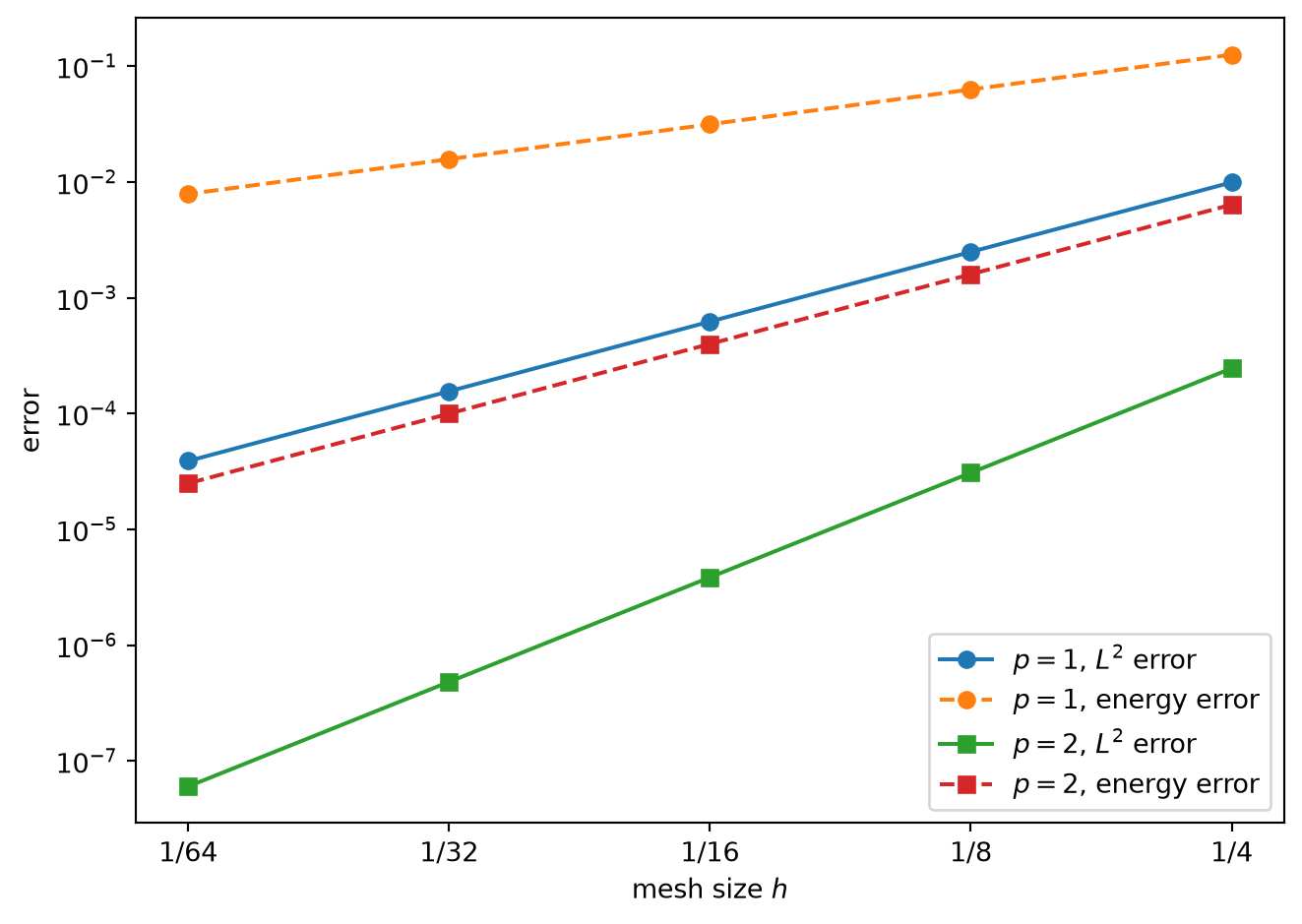
The printed rates approach \(2\) in \(L^2\) and \(1\) in the energy norm for linear elements, and \(3\) and \(2\) for quadratic elements. These are the values \(p+1\) and \(p\) predicted by Theorem 7.5 and Theorem 7.4 for a solution in \(H^{p+1}(0,1)\). The two error curves for each degree in Figure 7.7 are parallel to lines of slope \(p+1\) and \(p\).
Two common difficulties are worth anticipating. First, an observed rate computed from very coarse meshes may differ noticeably from the asymptotic value because the leading term \(Ch^r\) does not yet dominate. The rate should be judged from the trend of several successive refinements. Second, on very fine meshes, rounding error in the linear solve eventually stops the decrease of the error. For high-order elements this can occur at moderate mesh sizes, and it should not be mistaken for a loss of convergence.
Exercise 7.8 (Extending the convergence study) Use the program in Example 7.5.
- Add the cubic reference basis from Equation 5.58 with nodes \(-1,-1/3,1/3,1\). Before running, state the rates predicted by Theorem 7.4 and Theorem 7.5, and then confirm them.
- For \(p=1\), compute \(\max_i|u(x_i)-U_i|\) over the mesh nodes. Explain the result using 2, and explain why this quantity is not a suitable error measure for a convergence study.
- Replace the uniform nodes by nonuniform nodes whose interior points are moved by a random fraction, at most one quarter, of the uniform spacing, keeping the endpoints fixed and using a fixed random seed so that the study is reproducible. Use \(h=\max_e h_e\) in Equation 7.38 and check whether the rates change. Then use the elementwise estimate Equation 7.19 to explain why the global bound is stated with the largest element size \(h\).
- For \(p=2\), replace the six-point quadrature rule by the one-point rule in the assembly of \(\bF\) only. Compute the resulting \(L^2\)- and energy-error rates and compare them with the rates obtained using the six-point rule. Explain the change in terms of the variational crimes discussed after
7.9 Example of linear elasticity
Linear elasticity provides a vector-valued example of the analysis developed in this chapter. We first identify the continuity and coercivity constants in Céa’s lemma. We then examine two computations with linear triangular elements. A manufactured solution on a square verifies the rates predicted for a smooth displacement, whereas an L-shaped domain shows what changes when a reentrant corner limits the regularity of the solution.
7.9.1 Error estimates and their constants
The arguments used for the diffusion problem require a Hilbert space, a continuous and coercive bilinear form, a conforming finite element space, and an interpolation estimate. Linear elasticity has the same abstract structure, with constants determined by the elasticity tensor and Korn’s inequality.
Take homogeneous displacement data on \(\Gam_u\), so that the trial and test spaces coincide with \(\mathcal V_0\) in Equation 4.34, and let \(\bu_h\) solve the discrete problem Equation 6.69 in the vector Lagrange space Equation 6.67 with the same homogeneous data. Conformity gives Galerkin orthogonality,
\[ a_{\mathrm{el}}(\bu-\bu_h,\bv_h)=0 \qquad\forall\bv_h\in\mathcal V_{h,0}, \]
with \(a_{\mathrm{el}}\) from Equation 4.38. The continuity constant in Equation 4.40 is \(C_{\mathbb C}\), and the coercivity constant in Equation 4.42 is \(c_{\mathbb C}/C_K^2\), where \(C_K\) is the Korn constant of Theorem 4.1. Céa’s lemma therefore gives
\[ \norm{\bu-\bu_h}_{H^1(\Om;\R^d)} \leq \frac{C_{\mathbb C}C_K^2}{c_{\mathbb C}} \inf_{\bv_h\in\mathcal V_{h,0}} \norm{\bu-\bv_h}_{H^1(\Om;\R^d)} . \tag{7.39}\]
When \(\mathbb C\) has the major symmetry, \(a_{\mathrm{el}}\) is symmetric and defines the energy norm
\[ \norm{\bv}_{a_{\mathrm{el}}}^2 = \int_\Om\beps(\bv):\mathbb C:\beps(\bv)\,\dx , \]
which is twice the stored strain energy of the displacement field \(\bv\). The finite element displacement is then the best approximation in this norm, and by Equation 7.12 applied to Equation 4.43 it minimizes the total potential energy over the discrete space.
Galerkin orthogonality also gives a statement familiar from structural analysis. The elasticity analogue of Equation 7.11 follows from the same expansion with \(a_{\mathrm{el}}\) in place of \(a\):
\[ \norm{\bu-\bv_h}_{a_{\mathrm{el}}}^2 = \norm{\bu-\bu_h}_{a_{\mathrm{el}}}^2 + \norm{\bu_h-\bv_h}_{a_{\mathrm{el}}}^2 \qquad\forall\bv_h\in\mathcal V_{h,0}. \]
Taking \(\bv_h=\bm 0\) in this identity shows \(\norm{\bu_h}_{a_{\mathrm{el}}}\leq\norm{\bu}_{a_{\mathrm{el}}}\). Taking the test function equal to the solution in the continuous and discrete problems gives \(\ell_{\mathrm{el}}(\bu)=\norm{\bu}_{a_{\mathrm{el}}}^2\) and \(\ell_{\mathrm{el}}(\bu_h)=\norm{\bu_h}_{a_{\mathrm{el}}}^2\). Therefore
\[ \ell_{\mathrm{el}}(\bu_h) \leq \ell_{\mathrm{el}}(\bu). \tag{7.40}\]
The quantity \(\ell_{\mathrm{el}}(\bu)\) is the work done by the applied loads, called the compliance. With homogeneous displacement conditions, a conforming displacement-based finite element model underestimates both the compliance and the stored strain energy. In this global sense the discrete model is too stiff: restricting the displacements to a subspace reduces the work done by the loads. The inequality concerns these energy quantities; it does not imply that every displacement component is underestimated at every point.
Each displacement component of the vector Lagrange space is interpolated by the scalar interpolant. On a shape-regular family of affine simplicial meshes, applying Theorem 7.3 componentwise, under the assumption \(\bu\in H^s(\Om;\R^d)\) with \(2\leq s\leq p+1\), gives
\[ \norm{\bu-\bu_h}_{H^1(\Om;\R^d)} \leq C\,\frac{C_{\mathbb C}C_K^2}{c_{\mathbb C}}\;h^{s-1} \seminorm{\bu}_{H^s(\Om;\R^d)}, \]
where \(C\) depends on \(C_I\) and on an upper bound for \(h\). The upper bound enters because the full \(H^1\) norm combines an \(L^2\) interpolation term of order \(h^s\) with a gradient term of order \(h^{s-1}\). Since the strain is the symmetric part of the displacement gradient, \(\norm{\beps(\bv)}_{L^2}\leq\norm{\grad\bv}_{L^2}\). The stress error therefore satisfies
\[ \norm{\bsig-\bsig_h}_{L^2(\Om;\R^{d\times d})} = \norm{\mathbb C:\beps(\bu-\bu_h)}_{L^2(\Om;\R^{d\times d})} \leq C_{\mathbb C}\norm{\bu-\bu_h}_{H^1(\Om;\R^d)} , \]
and converges at the same rate as the displacement gradient. For the constant-strain triangle of Chapter 6 this rate is \(O(h)\). Under an \(H^2\) regularity assumption for the elasticity dual problem, analogous to Definition 7.4, the duality argument gives \(\norm{\bu-\bu_h}_{L^2(\Om;\R^d)}=O(h^{p+1})\) for smooth solutions.
The constant in Equation 7.39 depends on the material. For a homogeneous isotropic material with \(\lambda\geq0\) and \(\mu>0\), Equation 4.25 gives
\[ |\bm A:\mathbb C:\bm B| \leq (d\lambda+2\mu)\norm{\bm A}_F\norm{\bm B}_F, \qquad \bm A:\mathbb C:\bm A\geq2\mu\norm{\bm A}_F^2 \]
for symmetric tensors, so that \(C_{\mathbb C}/c_{\mathbb C}= 1+d\lambda/(2\mu)\). As Poisson’s ratio approaches \(1/2\), \(\lambda/\mu\) grows without bound, and so does the constant in Equation 7.39. The estimate remains true, but it no longer gives a bound independent of the material. The coercivity constant does not deteriorate; the growth comes from the continuity constant. For low-order displacement elements, the loss is real rather than an artifact of the proof: computed stresses for nearly incompressible materials show unphysical oscillations, more severe for linear than for quadratic elements (Arnold 2018, 155–57). Volumetric locking is the excessive stiffness caused by the displacement space being unable to satisfy the near-incompressibility constraint without severely restricting deformation. Stress oscillations can accompany this loss of accuracy. Mixed formulations require compatible approximation spaces; adding a pressure unknown alone does not ensure a remedy.
Exercise 7.9 (Material dependence of the elasticity estimate) Consider a homogeneous isotropic material in \(d\) dimensions with \(\lambda\geq0\) and \(\mu>0\).
- For symmetric \(\bm A\) and \(\bm B\), show that \(|\tr\bm A|\leq\sqrt d\,\norm{\bm A}_F\), and use it to prove \(|\bm A:\mathbb C:\bm B|\leq(d\lambda+2\mu)\norm{\bm A}_F\norm{\bm B}_F\).
- Prove \(\bm A:\mathbb C:\bm A\geq2\mu\norm{\bm A}_F^2\).
- Using Equation 4.26, write \(C_{\mathbb C}/c_{\mathbb C}\) as a function of \(\nu\) for \(d=3\), and evaluate it for \(\nu=0.3\), \(0.49\), and \(0.499\).
- Explain why Equation 7.40 holds for every \(\nu<1/2\) but gives no information about how large \(\ell_{\mathrm{el}}(\bu)-\ell_{\mathrm{el}}(\bu_h)\) is.
7.9.2 A smooth manufactured-solution example
We now verify the estimates with a problem for which the exact displacement is known. Let
\[ \Om=(0,1)^2, \qquad \Gam_u=\partial\Om, \]
and consider plane strain with Lamé parameters \(\lambda=\mu=1\). The stress is
\[ \bsig(\bu) =2\mu\beps(\bu) +\lambda\tr\!\left(\beps(\bu)\right)\bm I. \]
We prescribe \(\bu=\bm 0\) on \(\partial\Om\), take \(\rho=1\), and choose the exact displacement
\[ \bu_\star(x_1,x_2) = \begin{bmatrix} \sin(\pi x_1)\sin(\pi x_2)\\ \sin(2\pi x_1)\sin(\pi x_2) \end{bmatrix}. \tag{7.41}\]
Both components vanish on the boundary. Defining the body force by
\[ \bb=-\divg\bsig(\bu_\star) \tag{7.42}\]
ensures that \(\bu_\star\) satisfies the strong equilibrium equation. For the chosen Lamé parameters, the two components of this force are
\[ \begin{aligned} b_1 &=4\pi^2\left[ \sin(\pi x_1)\sin(\pi x_2) -\cos(2\pi x_1)\cos(\pi x_2) \right],\\ b_2 &=\pi^2\left[ 7\sin(2\pi x_1)\sin(\pi x_2) -2\cos(\pi x_1)\cos(\pi x_2) \right]. \end{aligned} \]
The variational problem is to find \(\bu\in\mathcal V_0=H^1_0(\Om;\R^2)\) such that
\[ a_{\mathrm{el}}(\bu,\bv) =\int_\Om\bsig(\bu):\beps(\bv)\,\dx =\int_\Om\bb\cdot\bv\,\dx \qquad\forall\bv\in\mathcal V_0. \tag{7.43}\]
The domain is divided into a uniform triangular mesh, and \(\bu_h\) is computed in the vector-valued \(P_1\) space. Since \(\bu_\star\) is smooth but is not a piecewise-linear function, the three errors
\[ \norm{\bu_\star-\bu_h}_{L^2(\Om;\R^2)}, \qquad \seminorm{\bu_\star-\bu_h}_{H^1(\Om;\R^2)}, \qquad \norm{\bu_\star-\bu_h}_{a_{\mathrm{el}}} \]
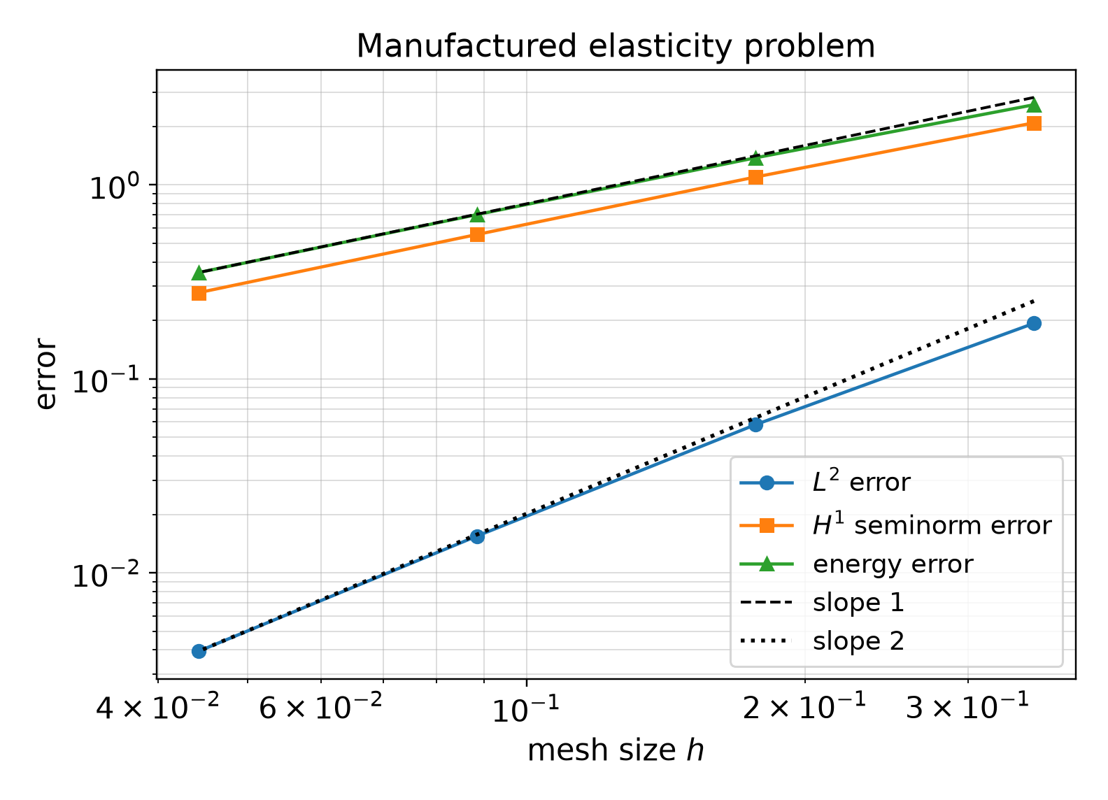
are nonzero and can be evaluated directly. For \(P_1\) elements, Theorem 7.4 predicts first-order convergence in the \(H^1\) seminorm and energy norm. The duality estimate predicts second-order convergence in the \(L^2\) norm, provided the elasticity dual problem has the required \(H^2\) regularity. In the table below, these three errors are denoted by \(E_0\), \(E_1\), and \(E_a\), respectively.
| \(n\) | \(h\) | \(E_0\) | Rate | \(E_1\) | Rate | \(E_a\) | Rate |
|---|---|---|---|---|---|---|---|
| 4 | \(0.353553\) | \(0.193111\) | – | \(2.087641\) | – | \(2.587643\) | – |
| 8 | \(0.176777\) | \(0.057978\) | 1.74 | \(1.096998\) | 0.93 | \(1.378080\) | 0.91 |
| 16 | \(0.088388\) | \(0.015447\) | 1.91 | \(0.554348\) | 0.98 | \(0.701988\) | 0.97 |
| 32 | \(0.044194\) | \(0.003933\) | 1.97 | \(0.277811\) | 1.00 | \(0.352746\) | 0.99 |
The observed rate is computed with Equation 7.38. The rates approach \(2\) in the \(L^2\) norm and \(1\) in both derivative-based norms. The first pair of meshes has not yet reached the asymptotic range, which is why its rates are farther from the predicted values. The log–log curves in Figure 7.8 show the same behavior.
7.9.3 An L-shaped domain with a reentrant corner
The preceding example was designed to satisfy the regularity assumptions of the estimates. We next keep the same material model and linear triangular elements but change the geometry. Let
\[ \Om=(-1,1)^2\setminus\bigl([0,1]\times[-1,0]\bigr). \]
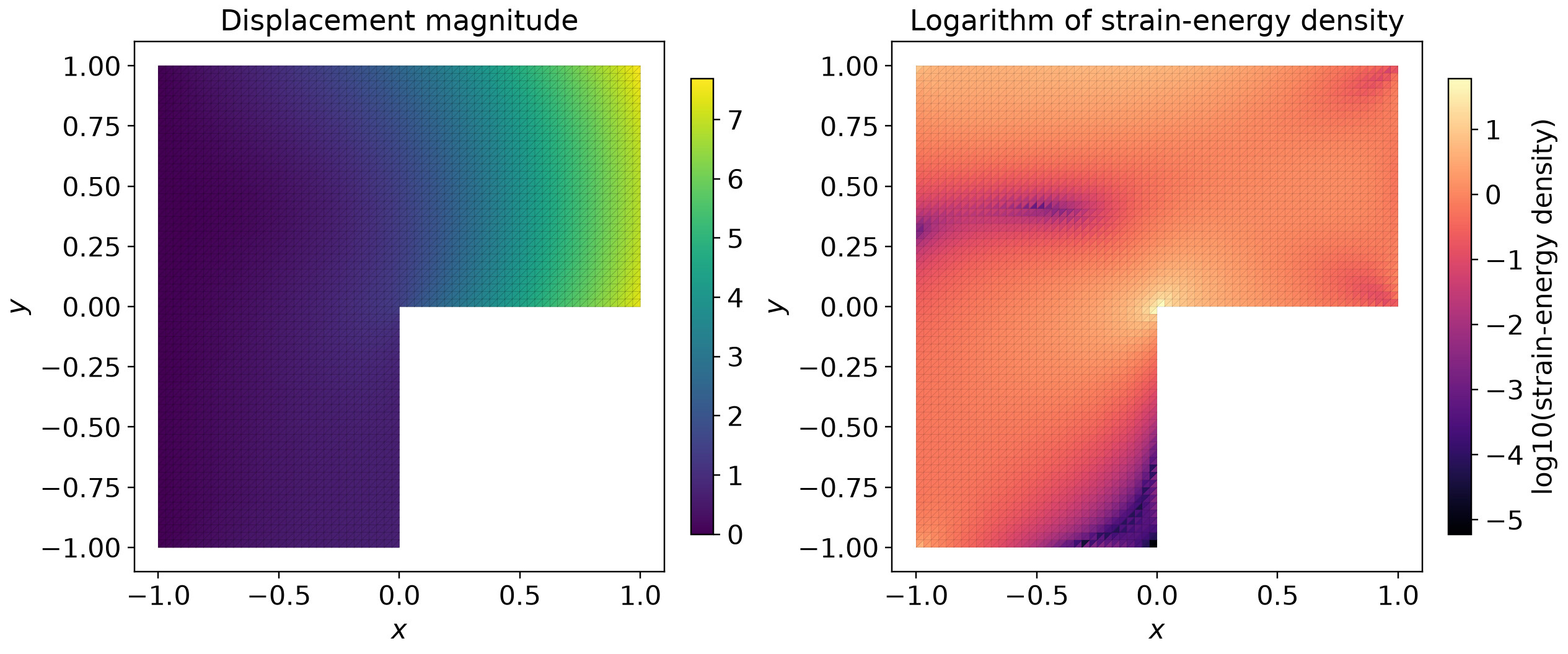
This L-shaped domain has a reentrant corner at the origin. The displacement is fixed on the left boundary,
\[ \bu=\bm 0 \qquad\text{on }\{(x_1,x_2)\in\partial\Om:x_1=-1\}, \]
and the downward traction \(\overline{\bt}=(0,-1)\) is prescribed on the right-hand segment \(x_1=1\), \(0\leq x_2\leq1\). The remaining boundary is traction free, and no body force is applied.
An exact displacement is not known for this problem, so the difference \(\bu-\bu_h\) cannot be evaluated. The computation instead compares solutions on nested meshes. The displacement magnitude and strain-energy density on the finest mesh are shown in Figure 7.9. The energy density is strongly concentrated near the reentrant corner.
Let \(\bu_{2h}\) be the solution on a coarse mesh and let \(\bu_h\) be the solution after uniform refinement. Because the meshes are nested, \(\bu_{2h}\in\mathcal V_{h,0}\). Testing the fine-mesh problem with \(\bu_{2h}\) gives \(a_{\mathrm{el}}(\bu_h,\bu_{2h})=\ell_{\mathrm{el}}(\bu_{2h})\). Using the discrete problem on the coarse mesh then yields
\[ \begin{aligned} d_h^2 :=\norm{\bu_h-\bu_{2h}}_{a_{\mathrm{el}}}^2 &=a_{\mathrm{el}}(\bu_h-\bu_{2h},\bu_h-\bu_{2h})\\ &=\ell_{\mathrm{el}}(\bu_h)-\ell_{\mathrm{el}}(\bu_{2h}). \end{aligned} \tag{7.44}\]
Thus \(d_h\) can be computed without knowing the exact solution. It is a successive-mesh difference, not the exact energy error. If the computation is in an asymptotic range and the exact error behaves like \(Ch^r\), the successive differences are expected to exhibit the same rate \(r\).
| Fine-mesh size \(h\) | Successive-mesh difference \(d_h\) | Observed rate |
|---|---|---|
| \(0.176777\) | \(0.848985\) | – |
| \(0.088388\) | \(0.542757\) | 0.65 |
| \(0.044194\) | \(0.337519\) | 0.69 |
For a displacement in \(H^2(\Om;\R^2)\), the \(P_1\) estimate obtained above would give
\[ \norm{\bu-\bu_h}_{a_{\mathrm{el}}} \leq Ch\seminorm{\bu}_{H^2(\Om;\R^2)}. \]
The rates in the table are below the smooth-solution rate \(1\). This result is consistent with the loss of regularity caused by the reentrant corner; it is not an exact-error study because \(\bu\) is unknown. At the same time, the largest elementwise strain-energy density increases under refinement. The two trends are shown together in Figure 7.10.
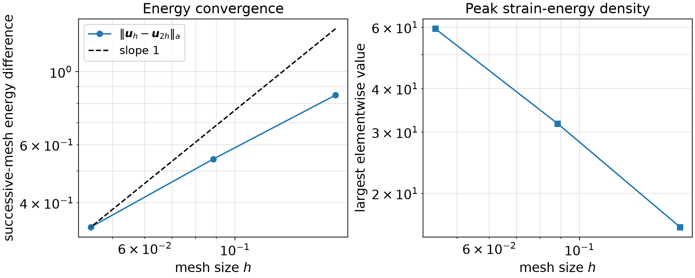
The example distinguishes global convergence from local field behavior. The decreasing successive-mesh differences provide evidence of global energy convergence, but a stress or strain quantity near the corner can remain poorly resolved on a uniform mesh. Chapter 8 develops residual error indicators and local mesh refinement for problems with this type of localized behavior.
7.10 Chapter summary
- Galerkin orthogonality states that the error is orthogonal to the conforming discrete test space in the bilinear form. Céa’s lemma then bounds the error by \(M/\alpha\) times the best approximation error.
- When the bilinear form is symmetric, the finite element solution is the best approximation in the energy norm and minimizes the energy over the discrete space.
- For linear elements in one dimension, interpolation errors are of order \(h^2\) in \(L^2\) and \(h\) in the \(H^1\) seminorm. In several dimensions, analogous estimates require a shape-regular mesh family.
- For degree-\(p\) elements and \(u\in H^s(\Om)\) with \(2\leq s\leq p+1\), the energy and \(H^1\) errors are of order \(h^{s-1}\). The attainable rate is limited by both the polynomial degree and the available regularity of the exact solution.
- The Aubin–Nitsche duality argument gives one additional power of \(h\) in the \(L^2\) estimate when the associated dual problem has \(H^2\) regularity.
- A convergence study requires integrated error norms and several mesh refinements. The smooth manufactured elasticity problem recovers the predicted \(P_1\) rates of two in \(L^2\) and one in the \(H^1\) seminorm and energy norm.
- For linear elasticity, the constants depend on the elastic moduli and Korn’s inequality. A reentrant corner can reduce the observed convergence rate and produce a localized strain-energy concentration. Near incompressibility increases the continuity-to-coercivity ratio and can cause volumetric locking in low-order displacement elements.