8 A Posteriori Error Estimation and Adaptive Finite Elements
Chapter 7 explained how the finite element error depends on the mesh size, the polynomial degree, and the smoothness of the exact solution. Its estimates predict convergence rates, but they do not supply the size of the error in a particular computation. The bound Equation 7.31 contains the seminorm \(\seminorm{u}_{H^s(\Om)}\) of the unknown solution and an interpolation constant \(C_I\) that is rarely known sharply. Chapter 7 also showed that the guaranteed rate depends on the smoothness of \(u\). On a polygon with a reentrant corner the solution may fail to belong to \(H^2(\Om)\), so the rate guaranteed for a smooth solution need not be attained by uniform refinement.
This chapter uses the computed solution \(u_h\) to obtain information about the error \(u-u_h\). An a posteriori error estimator is a quantity computed from \(u_h\), the data, and the mesh that is used to bound or approximate the error. Such an estimator has two uses. Its global value indicates whether the computation is accurate enough to stop. Its distribution over the elements indicates where the mesh should be refined. The second use leads to adaptive finite element methods, in which the mesh is refined only where the estimated error is large.
The chapter develops the residual-based estimator for scalar diffusion. The starting point is the residual of the variational equation, which Chapter 7 introduced in the discussion of Galerkin orthogonality. We first show that the energy-norm error is determined exactly by this residual. Integration by parts on each element then splits the residual into contributions from the element interiors, from the facets shared by neighboring elements, and from the Neumann boundary. To turn this identity into an error bound, we subtract a discrete test function using Galerkin orthogonality. A local averaging approximation makes the remaining test function small on each element and facet. Its approximation estimates supply the mesh-size weights; Cauchy–Schwarz then collects the weighted residuals into a computable estimator. This proves reliability. We then calculate the indicators, use them to mark elements, refine the mesh, and repeat the computation. Additional properties and extensions are summarized near the end of the chapter.
8.1 Why estimate the error after the computation
The elementwise interpolation estimate Equation 7.19 already suggests where a mesh should be fine. On an interval, it bounds the squared gradient error by
\[ \sum_{e=1}^{N_e}h_e^2\norm{u''}_{L^2(\mathcal K_e)}^2 . \]
An element contributes much to this sum when it is large or when \(|u''|\) is large on it. To reduce the bound with the fewest additional elements, one should make the elements small where \(|u''|\) is large and leave them large elsewhere. The difficulty is that \(u''\) is a property of the unknown exact solution. A mesh designed from this bound would require the answer before the computation.
The same difficulty appears in two and three dimensions. As Chapter 7 noted, the solution of a Laplace problem on a polygon with a reentrant corner may fail to belong to \(H^2(\Om)\). The reduced regularity is localized near the corner, where the derivatives may be large. Uniform refinement reduces the element size everywhere, including the large region in which the solution is smooth and the error is already small. Most of the additional unknowns are therefore spent where they reduce the error least.
An a posteriori estimator replaces the unknown quantities in such bounds by quantities that can be evaluated once \(u_h\) has been computed. This chapter uses the estimator in an iterative procedure:
- solve the discrete problem on the current mesh;
- estimate the error from the computed solution;
- mark the elements with the largest estimated contributions; and
- refine the marked elements and repeat.
This is the solve–estimate–mark–refine loop. The following sections develop the error estimator and its bounds before returning to marking and refinement.
8.2 The residual and the error
8.2.1 Setting
We use the scalar diffusion problem and the finite element discretization of Section 7.1. Thus \(\Om\subset\R^d\), \(d\in\{2,3\}\), is a bounded polygonal or polyhedral domain, \(\Gam_D\) has positive boundary measure, the coefficient satisfies Equation 3.8, \(f\in L^2(\Om)\), \(q\in L^2(\Gam_N)\), and \(g=0\). Denote the exact solution by \(u\in\Vzero\) and the finite element solution by \(u_h\in\Vhzero\). Their variational equations are recalled below. We retain the mesh and discretization assumptions of Chapter 7: the mesh is conforming and boundary fitted and resolves the partition into \(\Gam_D\) and \(\Gam_N\), \(\Vh\) is the continuous Lagrange space of degree \(p\geq1\), and the forms are evaluated exactly. In addition, we assume that
- \(\Th\) belongs to a shape-regular family of affine simplicial meshes in the sense of Definition 7.3, with shape bound \(\sigma\); and
- the coefficient is smooth on each element, in the sense that \(k|_{\mathcal K_e}\in C^1(\overline{\mathcal K_e})\) for every \(\mathcal K_e\in\Th\).
The elementwise regularity assumption allows \(k\) to jump across facets, as it does at an interface between two materials, provided that the mesh is aligned with the interface. It is needed because the estimator below contains \(\divg(k\grad u_h)\) on each element and the normal component of \(k\grad u_h\) on each facet. In the most common case, \(k\) is constant on each element.
For reference, the spaces and forms are
\[ \begin{aligned} \Vzero&=\{v\in H^1(\Om):v=0\text{ on }\Gam_D\}, &\Vhzero&=\Vh\cap\Vzero,\\ a(w,v)&=\int_\Om k\grad w\cdot\grad v\,\dx,\\ \ell(v)&=\int_\Om fv\,\dx+\int_{\Gam_N}qv\,\ds. \end{aligned} \tag{8.1}\]
Thus \(a(u,v)=\ell(v)\) for every \(v\in\Vzero\), and \(a(u_h,v_h)=\ell(v_h)\) for every \(v_h\in\Vhzero\). The energy norm is \(\norm{v}_a=\sqrt{a(v,v)}\). The normal datum follows the convention of Chapter 3: \(\bq=k\grad u\) and \(q=\bq\cdot\bn\) on \(\Gam_N\).
8.2.2 The residual functional
Chapter 7 observed that, for any \(w\in\Vzero\), the linear functional \(v\mapsto\ell(v)-a(w,v)\) measures how far \(w\) is from satisfying the variational equation. We now give this functional a name for \(w=u_h\).
Definition 8.1 (Residual of the finite element solution) The residual of \(u_h\) is the linear functional \(R(u_h;\cdot):\Vzero\to\R\) defined by
\[ R(u_h;v) = \ell(v)-a(u_h,v) \qquad\forall v\in\Vzero . \tag{8.2}\]
For a given test function \(v\), the number \(R(u_h;v)\) can be computed. It requires only the data \(f\), \(q\), and \(k\) and the computed solution \(u_h\); the exact solution does not appear. The residual is also continuous on \(\Vzero\). The bound Equation 3.25 shows that \(\ell\) is continuous, and Equation 3.23 shows that \(v\mapsto a(u_h,v)\) is continuous. Hence \(R(u_h;\cdot)\) belongs to the dual space \(\Vzero^*\) of Definition 2.22.
8.2.3 The error–residual relation
The exact solution satisfies \(a(u,v)=\ell(v)\) for every \(v\in\Vzero\). Substituting \(\ell(v)=a(u,v)\) into Equation 8.2 and using linearity of \(a\) in its first argument gives
\[ R(u_h;v) = a(u,v)-a(u_h,v) = a(e,v) \qquad\forall v\in\Vzero, \tag{8.3}\]
where \(e=u-u_h\). This identity connects a computable functional with the unknown error. It has two immediate consequences.
First, every discrete test function is also an admissible test function in Equation 8.3. Galerkin orthogonality Equation 7.10 therefore states that the residual vanishes on the discrete test space:
\[ R(u_h;v_h)=0 \qquad\forall v_h\in\Vhzero . \tag{8.4}\]
In the assembly notation of Chapters 5 and 6, substitution of \(u_h=\sum_jU_j\phi_j\) into the residual gives, for each free basis function,
\[ R(u_h;\phi_i)=F_i-\sum_jK_{ij}U_j=0. \tag{8.5}\]
This is the corresponding entry of the algebraic residual \(\bR=\bF-\bK\bU\). The discrete equations say nothing about the residual on functions outside \(\Vhzero\). In general, \(R(u_h;v)\neq0\) for such functions, and the residual vanishes on all of \(\Vzero\) only when \(u_h=u\).
Second, the energy norm of the error is the dual norm of the residual when test functions are measured in the energy norm. Since the diffusion form is symmetric and coercive, \(a\) is an inner product on \(\Vzero\) with associated norm \(\norm{\cdot}_a\) from Definition 7.1. The Cauchy–Schwarz inequality for this inner product and Equation 8.3 give
\[ |R(u_h;v)| = |a(e,v)| \leq \norm{e}_a\norm{v}_a \qquad\forall v\in\Vzero . \]
If \(e\neq0\), the choice \(v=e\) gives equality, because \(R(u_h;e)=a(e,e)=\norm{e}_a^2\). Therefore
\[ \norm{u-u_h}_a = \sup_{v\in\Vzero,\,v\neq0} \frac{|R(u_h;v)|}{\norm{v}_a}. \tag{8.6}\]
If \(e=0\), the residual vanishes on all of \(\Vzero\), and both sides are zero.
Equation 8.6 is exact, but it is not yet an estimate that can be evaluated. The supremum is taken over the infinite-dimensional space \(\Vzero\), and the maximizing test function is the unknown error itself. The remainder of the derivation replaces this supremum by an upper bound built from local, computable quantities.
The same idea can be expressed in the \(H^1(\Om)\) norm. With the continuity and coercivity constants \(M\) and \(\alpha\) of Equation 7.3 and Equation 7.4, and the dual norm Equation 2.57 taken with respect to \(\norm{\cdot}_{H^1(\Om)}\),
\[ \frac{1}{M}\norm{R(u_h;\cdot)}_{\Vzero^*} \leq \norm{u-u_h}_{H^1(\Om)} \leq \frac{1}{\alpha}\norm{R(u_h;\cdot)}_{\Vzero^*} \tag{8.7}\]
(Arnold 2018, 71). The energy norm gives equality because it is the norm defined by the bilinear form. We work with the energy norm in what follows.
Exercise 8.1 (The residual in the \(H^1\) norm)
- Use Equation 8.3 and Equation 7.3 to prove the lower bound in Equation 8.7.
- Take \(v=e\) in Equation 8.3 and use Equation 7.4 to prove the upper bound.
- For the diffusion problem, use Equation 7.5 to write the ratio of the two constants in Equation 8.7. Explain why Equation 8.6 contains no such ratio.
8.3 Element and facet residuals
The residual Equation 8.2 is a single functional on the whole domain. To identify where the error originates, we rewrite it as a sum of contributions from individual elements and facets. The rewriting uses integration by parts on each element. It requires notation for the facets of the mesh.
8.3.1 Facets, normals, and jumps
Recall from Section 6.1 that the boundary of an element consists of facets: edges in two dimensions and faces in three dimensions. Let \(\mathcal F_h\) denote the set of all facets of \(\Th\). Because the mesh is conforming and resolves the boundary partition, each facet belongs to exactly one of three classes:
- \(\mathcal F_h^{\mathrm{int}}\), the interior facets, each shared by two elements;
- \(\mathcal F_h^{D}\), the boundary facets contained in \(\overline{\Gam_D}\); and
- \(\mathcal F_h^{N}\), the boundary facets contained in \(\overline{\Gam_N}\).
For a facet \(\mathcal F\), let \(h_{\mathcal F}=\operatorname{diam}(\mathcal F)\). On a shape-regular mesh, \(h_{\mathcal F}\) and the diameter \(h_e\) of an element containing \(\mathcal F\) are comparable, with constants depending only on \(\sigma\) and \(d\).
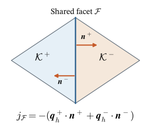
An interior facet \(\mathcal F\) is shared by two elements, which we label \(\mathcal K^+\) and \(\mathcal K^-\). Let \(\bn_{\mathcal F}\) be the unit normal to \(\mathcal F\) pointing from \(\mathcal K^+\) into \(\mathcal K^-\). Thus \(\bn_{\mathcal F}\) is the outward normal of \(\mathcal K^+\) on \(\mathcal F\), and \(-\bn_{\mathcal F}\) is the outward normal of \(\mathcal K^-\). For a boundary facet, \(\bn_{\mathcal F}=\bn\) is the outward unit normal of \(\Om\).
A finite element function is a polynomial on each element, but its gradient is generally discontinuous across facets. For a function \(w\) whose restrictions to \(\mathcal K^+\) and \(\mathcal K^-\) have traces \(w^+\) and \(w^-\) on \(\mathcal F\), the jump across \(\mathcal F\) is
\[ [\![w]\!]_{\mathcal F} = w^+-w^- \qquad\text{on }\mathcal F . \tag{8.8}\]
The labels \(\mathcal K^+\) and \(\mathcal K^-\) are arbitrary. Exchanging them changes the sign of the jump, but it also reverses \(\bn_{\mathcal F}\). The quantity used below, \([\![k\grad u_h\cdot\bn_{\mathcal F}]\!]_{\mathcal F}\), contains both factors and is therefore unchanged by the choice of labels.
Following Equation 3.6, define the discrete flux
\[ \bq_h=k\grad u_h \qquad\text{on each element }\mathcal K_e . \tag{8.9}\]
It is defined element by element. Under the elementwise regularity assumption, and because \(u_h\) is a polynomial on each affine element, \(\bq_h|_{\mathcal K_e}\) is continuously differentiable on \(\overline{\mathcal K_e}\). Its normal component on a facet is therefore defined from each side.
Writing the two outward normals as \(\bn^+=\bn_{\mathcal F}\) and \(\bn^-=-\bn_{\mathcal F}\) makes the normal-flux jump explicit:
\[ [\![\bq_h\cdot\bn_{\mathcal F}]\!]_{\mathcal F} =\bq_h^+\cdot\bn_{\mathcal F}-\bq_h^-\cdot\bn_{\mathcal F} =\bq_h^+\cdot\bn^++\bq_h^-\cdot\bn^-. \tag{8.10}\]
Exchanging the element labels only exchanges the two terms in the last sum. Unlike the signed jump of a scalar field alone, this normal-flux sum is independent of the labeling.
8.3.2 Integration by parts on each element
Start from the residual Equation 8.2 with the diffusion forms Equation 3.18:
\[ R(u_h;v) = \int_\Om fv\,\dx +\int_{\Gam_N}qv\,\ds -\int_\Om k\grad u_h\cdot\grad v\,\dx \qquad\forall v\in\Vzero . \]
The elements have disjoint interiors, so the last integral is the sum of the integrals over the elements. On one element, apply Green’s formula Equation 2.39 with \(\Om\) replaced by \(\mathcal K_e\), the scalar field \(v\), and the vector field \(k\grad u_h\). With \(\bn_e\) the outward unit normal of \(\mathcal K_e\),
\[ \int_{\mathcal K_e}k\grad u_h\cdot\grad v\,\dx = -\int_{\mathcal K_e}\divg(k\grad u_h)\,v\,\dx +\int_{\partial\mathcal K_e}(k\grad u_h\cdot\bn_e)\,v\,\ds . \]
Chapter 2 stated Green’s formula for smooth fields. Here the vector field is continuously differentiable on \(\overline{\mathcal K_e}\), while \(v\in H^1(\mathcal K_e)\) is used through its weak derivatives and its trace on \(\partial\mathcal K_e\), as in the derivation of the weak form in Chapter 3. Summing over the elements gives
\[ \begin{aligned} R(u_h;v) ={}& \sum_{e=1}^{N_e}\int_{\mathcal K_e} \bigl(f+\divg(k\grad u_h)\bigr)v\,\dx\\ &-\sum_{e=1}^{N_e}\int_{\partial\mathcal K_e} (k\grad u_h\cdot\bn_e)\,v\,\ds +\int_{\Gam_N}qv\,\ds . \end{aligned} \tag{8.11}\]
The element boundary integrals are now regrouped facet by facet. Every facet of every element belongs to exactly one of the three classes above.
Facets on \(\Gam_D\). Every \(v\in\Vzero\) vanishes on \(\Gam_D\), so these facets contribute nothing.
Facets on \(\Gam_N\). Such a facet belongs to one element, whose outward normal is \(\bn\). Its contribution from the middle sum in Equation 8.11 combines with the part of the last integral over the same facet:
\[ -\int_{\mathcal F}(k\grad u_h\cdot\bn)\,v\,\ds +\int_{\mathcal F}qv\,\ds = \int_{\mathcal F}\bigl(q-k\grad u_h\cdot\bn\bigr)v\,\ds . \]
Interior facets. An interior facet appears twice in the middle sum: once from \(\mathcal K^+\), with outward normal \(\bn_{\mathcal F}\), and once from \(\mathcal K^-\), with outward normal \(-\bn_{\mathcal F}\). A function \(v\in H^1(\Om)\) has the same trace on \(\mathcal F\) from both elements. This is a standard property of \(H^1\) functions on a conforming mesh, which we use without proof. The two contributions therefore combine into
\[ -\int_{\mathcal F} \bigl(k^+\grad u_h^+\cdot\bn_{\mathcal F} -k^-\grad u_h^-\cdot\bn_{\mathcal F}\bigr)v\,\ds = -\int_{\mathcal F} [\![k\grad u_h\cdot\bn_{\mathcal F}]\!]_{\mathcal F}\,v\,\ds . \]
The surviving terms define the residuals that appear in the estimator.
Definition 8.2 (Element and facet residuals) The element residual on \(\mathcal K_e\in\Th\) is
\[ r_e = f+\divg(k\grad u_h) = f+\divg\bq_h \qquad\text{on }\mathcal K_e . \tag{8.12}\]
The facet residual on \(\mathcal F\in \mathcal F_h^{\mathrm{int}}\cup\mathcal F_h^{N}\) is
\[ j_{\mathcal F} = \begin{cases} -[\![k\grad u_h\cdot\bn_{\mathcal F}]\!]_{\mathcal F} =-[\![\bq_h\cdot\bn_{\mathcal F}]\!]_{\mathcal F}, & \mathcal F\in\mathcal F_h^{\mathrm{int}},\\[0.4em] q-k\grad u_h\cdot\bn =q-\bq_h\cdot\bn, & \mathcal F\in\mathcal F_h^{N}. \end{cases} \tag{8.13}\]
With these definitions, the facet-by-facet regrouping of Equation 8.11 gives the residual representation
\[ R(u_h;v) = \sum_{e=1}^{N_e}\int_{\mathcal K_e}r_e\,v\,\dx +\sum_{\mathcal F\in\mathcal F_h^{\mathrm{int}}\cup\mathcal F_h^{N}} \int_{\mathcal F}j_{\mathcal F}\,v\,\ds \qquad\forall v\in\Vzero . \tag{8.14}\]
This identity is exact. It holds for every admissible test function and makes no approximation of the data or of \(u_h\).
8.3.3 Interpretation of the residuals
Each residual measures a failure of \(u_h\) to satisfy one part of the strong problem of Chapter 3. The element residual is the defect in the balance equation \(-\divg(k\grad u)=f\) of Equation 3.5, evaluated in the interior of an element. In heat conduction it is the difference between the prescribed heat source and the net outward physical heat flow per unit volume; the physical heat-flow vector is \(-\bq_h\).
The interior facet residual is the negative jump in the normal component of \(\bq_h\), or equivalently the jump in physical heat flow. If the exact solution is regular enough on each element for the corresponding quantities to be defined, its normal flux is continuous across interior facets: the heat leaving one element through a facet enters its neighbor. The computed flux does not have this property, because \(\grad u_h\) is discontinuous across facets. The Neumann residual is the difference between the prescribed normal datum \(q\) and the computed component \(\bq_h\cdot\bn\). The Galerkin method satisfies both flux conditions only in the weak sense of Equation 8.4.
The two kinds of residual are not independent. Taking \(v=\phi_i\) for a free basis function in Equation 8.14 and using Equation 8.4 gives
\[ \sum_{e=1}^{N_e}\int_{\mathcal K_e}r_e\,\phi_i\,\dx +\sum_{\mathcal F\in\mathcal F_h^{\mathrm{int}}\cup\mathcal F_h^{N}} \int_{\mathcal F}j_{\mathcal F}\,\phi_i\,\ds =0 . \]
The discrete equations therefore balance the element and facet residuals against each other on every basis function. Neither kind of residual vanishes separately in general.
For linear elements, one simplification occurs often enough to state explicitly. If \(p=1\) and \(k\) is constant on each element, then \(\grad u_h\) and \(k\grad u_h\) are constant on each element, \(\divg(k\grad u_h)=0\), and the element residual reduces to \(r_e=f|_{\mathcal K_e}\). All information about the computed gradient then enters through the facet residuals.
Example 8.1 (Residuals for the axial bar) Consider the bar of Equation 5.2 with linear elements on \(\mathcal K_e=(x_e,x_{e+1})\), \(e=1,\ldots,N_e\), and assume that \(AE\) is smooth on each element. In one dimension, an element is an interval and its facets are its two endpoints. The interior facets are the interior nodes \(x_2,\ldots,x_{N_e}\), the facet at \(x_1=0\) carries the essential condition, and the facet at \(x_{N_n}=L\), with \(N_n=N_e+1\), carries the applied force \(\overline P\). A facet integral is the value of the integrand at the point.
Integrating by parts on each element in \(R(u_h;v)=\ell(v)-a(u_h,v)\) and using \(v(0)=0\) gives
\[ R(u_h;v) = \sum_{e=1}^{N_e}\int_{x_e}^{x_{e+1}}r_e\,v\,\dd x +\sum_{i=2}^{N_e}j_i\,v(x_i) +j_{N_n}\,v(L), \]
with
\[ \begin{aligned} r_e&=f+(AE\,u_h')',\\ j_i&=(AE\,u_h')(x_i^+)-(AE\,u_h')(x_i^-),\\ j_{N_n}&=\overline P-(AE\,u_h')(L^-), \end{aligned} \]
where \(x_i^-\) and \(x_i^+\) denote limits from the left and right. Here \(AE\,u_h'\) is the computed axial force. The interior residual \(j_i\) is its jump at node \(x_i\), which would have to be balanced by a concentrated nodal force that is not present in the loading. The boundary residual \(j_{N_n}\) is the mismatch between the applied end force and the computed end force. These expressions agree with Equation 8.12 and Equation 8.13: with \(\mathcal K^+\) the element to the left of a node, \(\bn_{\mathcal F}=+1\), and the bar’s natural condition \(AE\,u'(L)=\overline P\) corresponds to the normal datum \(q=\overline P\) at \(x=L\).
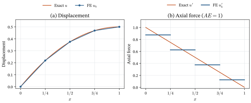
Now take the uniformly loaded bar of Example 5.5, with \(L=AE=f=1\), \(\overline P=0\), a uniform mesh of size \(h\), and exact solution \(u(x)=x-x^2/2\). The nodal-exactness example in Chapter 7 shows that \(u_h=\Ih u\). The slope of \(u_h\) on \(\mathcal K_e\) is the slope of the chord of a quadratic, which equals \(u'\) at the element midpoint \(\bar x_e\):
\[ u_h'|_{\mathcal K_e}=u'(\bar x_e)=1-\bar x_e . \]
Since \(u_h''=0\) on each element and \(f=1\),
\[ \begin{aligned} r_e&=1,\\ j_i&=\bigl(1-(x_i+\tfrac h2)\bigr)-\bigl(1-(x_i-\tfrac h2)\bigr)=-h,\\ j_{N_n}&=0-\bigl(1-(1-\tfrac h2)\bigr)=-\frac h2 . \end{aligned} \]
Every residual is nonzero, even though every nodal value of \(u_h\) is exact. The residuals detect the error between the nodes.
The balance on a basis function can be checked directly. For an interior node, \(\int_0^1 r\,\phi_i\,\dd x=h\), because \(r=1\) and the hat function has integral \(h\). The facet term is \(j_i\phi_i(x_i)=-h\), and the two cancel. For the last node, \(\int_0^1 r\,\phi_{N_n}\,\dd x=h/2\) and \(j_{N_n}=-h/2\). Both results agree with Equation 8.4.
Exercise 8.2 (A flux jump on two triangles) Let \(k=1\), and let \(\mathcal K^+\) and \(\mathcal K^-\) be the triangles with vertices \((0,0)\), \((1,0)\), \((1,1)\) and \((0,0)\), \((1,1)\), \((0,1)\), respectively. A continuous piecewise-linear function \(u_h\) has vertex values \(u_h(0,0)=0\), \(u_h(1,0)=1\), \(u_h(1,1)=1\), and \(u_h(0,1)=1\).
- Find \(u_h\) on each triangle and compute \(\grad u_h^+\) and \(\grad u_h^-\).
- Determine \(\bn_{\mathcal F}\) on the shared diagonal \(\mathcal F\), and compute \(j_{\mathcal F}\) from Equation 8.13.
- Exchange the labels \(\mathcal K^+\) and \(\mathcal K^-\) and recompute \(j_{\mathcal F}\). Use Equation 8.10 to explain why it is unchanged.
- Compute \(h_{\mathcal F}\norm{j_{\mathcal F}}_{L^2(\mathcal F)}^2\).
- Explain why the element residuals are \(r^\pm=f\) for any source \(f\).
8.4 Quasi-interpolation and local approximation
8.4.1 Using Galerkin orthogonality
The representation Equation 8.14 suggests bounding \(R(u_h;e)=\norm{e}_a^2\) term by term. Applying the Cauchy–Schwarz inequality directly to \(\int_{\mathcal K_e}r_e\,e\,\dx\) would produce \(\norm{r_e}_{L^2(\mathcal K_e)}\norm{e}_{L^2(\mathcal K_e)}\). Such a bound does not contain a power of the element size, so it gives no information about how the error is distributed relative to the mesh.
Galerkin orthogonality supplies the missing factor. By Equation 8.4, for every \(v\in\Vzero\) and every \(v_h\in\Vhzero\),
\[ R(u_h;v)=R(u_h;v-v_h). \tag{8.15}\]
If \(v_h\) is chosen as a good local approximation of \(v\), the difference \(v-v_h\) is small on each element, with a size proportional to the local mesh size. For the error bound, take \(v=e=u-u_h\). The two identities that we need to combine are therefore
\[ \norm{e}_a^2=R(u_h;e), \qquad R(u_h;e)=R(u_h;e-v_h) \quad\text{for every }v_h\in\Vhzero. \]
The task is to choose \(v_h\) so that \(e-v_h\) can be bounded using only first weak derivatives of \(e\). The function \(v_h\) is a tool in the proof; it will not have to be computed to evaluate the estimator.
The nodal interpolant of Chapter 7 cannot be used for this purpose in two and three dimensions. The function to be approximated will be the error \(e\), which is known only to belong to \(\Vzero\subset H^1(\Om)\). As explained in Section 7.5, a general \(H^1\) function need not have point values when \(d\geq2\), so \(\Ih e\) need not be defined. Operators that avoid point values, for example by averaging over a neighborhood of each node, are called quasi-interpolation operators. The Clément interpolant is the classical example (Arnold 2018, 67–70).
8.4.2 Approximating a function by local averages
First consider \(P_1\) elements, with the global nodal basis functions \(\phi_i\) already constructed in Chapter 6. For a continuous function \(v\), the nodal interpolant is \(\Ih v=\sum_i v(\bx_i)\phi_i\). We retain these basis functions but replace each point value by a local average.
For a mesh vertex \(\bx_i\), its vertex patch \(\omega_i\) is the interior of the union of the closures of all elements containing that vertex:
\[ \omega_i=\operatorname{int}\!\left( \bigcup_{\mathcal K_e:\,\bx_i\in\overline{\mathcal K_e}} \overline{\mathcal K_e}\right). \]
Thus \(\overline{\omega_i}=\operatorname{supp}\phi_i\). Its area in two dimensions, or volume in three dimensions, is denoted by \(|\omega_i|\). At a vertex not on the Dirichlet boundary, use the coefficient
\[ c_i(v)=\frac{1}{|\omega_i|}\int_{\omega_i}v\,\dx. \]
This integral is well defined for \(v\in H^1(\Om)\subset L^2(\Om)\): Cauchy–Schwarz gives \(|\int_{\omega_i}v\,\dx|\leq|\omega_i|^{1/2}\norm{v}_{L^2(\omega_i)}\). It does not require a value of \(v\) at \(\bx_i\).
At a Dirichlet vertex, set the coefficient to zero instead of taking the average. With \(N_v\) the number of mesh vertices, the averaging operator is
\[ \mathcal Q_hv=\sum_{i=1}^{N_v}c_i(v)\phi_i, \qquad c_i(v)=\begin{cases} |\omega_i|^{-1}\displaystyle\int_{\omega_i}v\,\dx, &\bx_i\notin\overline{\Gam_D},\\ 0,&\bx_i\in\overline{\Gam_D}. \end{cases} \tag{8.16}\]
Use the connectivity map \(I^e\) from Chapter 6: local vertex \(a\) of \(\mathcal K_e\) has global number \(I^e(a)\). By Equation 6.17, the global basis function \(\phi_{I^e(a)}\) restricts to \(\phi_a^e\) on that element. The restriction of the averaging approximation is therefore
\[ (\mathcal Q_hv)|_{\mathcal K_e} =\sum_{a=1}^{d+1}c_{I^e(a)}(v)\phi_a^e. \]
These coefficients come from the neighboring patches, not just from \(\mathcal K_e\). Two adjacent elements use the same coefficient at every shared vertex, so their linear restrictions agree along the shared facet. The result is continuous. On a Dirichlet facet every vertex coefficient is zero, so the restriction is zero there. Hence \(\mathcal Q_hv\in\Vhzero\).
This averaging version of the Clément operator is described in Schöberl (n.d.), §27.1. It need not agree with a continuous function at the vertices: \((\mathcal Q_hv)(\bx_i)=c_i(v)\), whereas \((\Ih v)(\bx_i)=v(\bx_i)\).
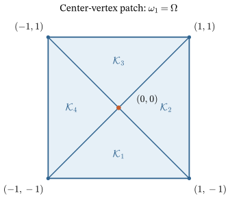
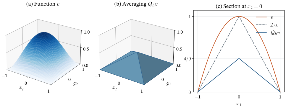
Example 8.2 (A patch average on four triangles) Partition \(\Om=(-1,1)^2\) into four triangles by joining its center to the four corners, use \(P_1\) elements, and impose zero values on the whole boundary. Let \(v(x_1,x_2)=(1-x_1^2)(1-x_2^2)\). The only free vertex is \(\bx_1=(0,0)\), and its patch is the whole square, of area four. Therefore
\[ \begin{aligned} c_1(v)&=\frac14\int_{-1}^1\int_{-1}^1 (1-x_1^2)(1-x_2^2)\,\dd x_1\,\dd x_2\\ &=\frac14\left(\left[t-\frac{t^3}{3}\right]_{-1}^1\right)^2 =\frac14\left(\frac43\right)^2=\frac49. \end{aligned} \]
All boundary coefficients are zero, so \(\mathcal Q_hv=\tfrac49\phi_1\). In contrast, \(\Ih v=\phi_1\) because \(v(0,0)=1\). Both satisfy the prescribed boundary values, but only the nodal interpolant agrees with \(v\) at the center.
On the bottom triangle, for example, \(\phi_1=1+x_2\), so \(\mathcal Q_hv=\tfrac49(1+x_2)\). On the other three triangles it is \(\tfrac49(1-x_1)\), \(\tfrac49(1-x_2)\), and \(\tfrac49(1+x_1)\), respectively. These four planes join continuously. Their common value at the center is \(4/9\), rather than \(v(0,0)=1\).
The approximation used in the proof need not have the same polynomial degree as \(u_h\). For \(p>1\), use the auxiliary \(P_1\) vertex basis \(\phi_i^{(1)}\) in Equation 8.16. The output is still in \(\Vhzero\), because every continuous piecewise-linear function belongs to the degree-\(p\) Lagrange space. This construction is used only to approximate test functions in the error analysis; it does not replace the degree-\(p\) space used to solve the PDE.
8.4.3 Local approximation estimates
We have constructed a discrete function. We next need a bound for the difference \(v-\mathcal Q_hv\), first over an element and then over a facet. The coefficients used on an element depend on all its vertices’ patches. This is why an estimate on one element involves a larger neighborhood.
For an element \(\mathcal K_e\), let the patch \(\omega_e\) be the union of the closed elements that share at least one vertex with \(\mathcal K_e\). For a facet \(\mathcal F\), let \(\omega_{\mathcal F}\) be the union of the closed elements that share at least one vertex with \(\mathcal F\). The seminorms \(\seminorm{\cdot}_{H^1(\omega_e)}\) and \(\seminorm{\cdot}_{H^1(\omega_{\mathcal F})}\) are defined by integrating over these patches.
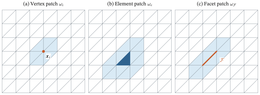
The left panel of Figure 8.5 is the patch used to compute one coefficient. The middle and right panels show the unions needed to bound the approximation on an element and on a facet. The local approximation property used below is the following.
Hypothesis (Q). There are a linear operator \(\mathcal Q_h:\Vzero\to\Vhzero\) and a constant \(C_Q\), depending only on \(d\), \(p\), and \(\sigma\), such that for every \(w\in\Vzero\), every element \(\mathcal K_e\in\Th\), and every facet \(\mathcal F\in\mathcal F_h^{\mathrm{int}}\cup\mathcal F_h^{N}\),
\[ \norm{w-\mathcal Q_hw}_{L^2(\mathcal K_e)} \leq C_Q\,h_e\,\seminorm{w}_{H^1(\omega_e)}, \tag{8.17}\]
\[ \norm{w-\mathcal Q_hw}_{L^2(\mathcal F)} \leq C_Q\,h_{\mathcal F}^{1/2}\,\seminorm{w}_{H^1(\omega_{\mathcal F})}. \tag{8.18}\]
For homogeneous Dirichlet conditions on the whole boundary, these estimates for the averaging operator are stated in Schöberl (n.d.), §27.1. The mixed-boundary reliability result below is conditional on Hypothesis (Q). It applies to any boundary-preserving operator with these two estimates, not only to the particular averaging formula. The following calculations explain the powers of \(h\) without attempting the full quasi-interpolation theory.
For \(p=1\) and an interior element, the reason for the element estimate can be seen directly from the construction. Its local basis functions satisfy \(\sum_{a=1}^{d+1}\phi_a^e=1\) and \(0\leq\phi_a^e\leq1\). Thus
\[ v-\mathcal Q_hv =\sum_{a=1}^{d+1}(v-c_{I^e(a)}(v))\phi_a^e \quad\text{on }\mathcal K_e. \]
Subtracting a mean removes the constant part of a function. The mean-value Poincaré estimate on a vertex patch bounds the remaining part by its gradient times the patch diameter. On a shape-regular mesh, that diameter is comparable with \(h_e\) for a vertex of \(\mathcal K_e\). Applying this estimate to each coefficient in the last sum gives
\[ \begin{aligned} \norm{v-\mathcal Q_hv}_{L^2(\mathcal K_e)} &\leq\sum_{a=1}^{d+1} \norm{v-c_{I^e(a)}(v)}_{L^2(\omega_{I^e(a)})}\\ &\leq C h_e\sum_{a=1}^{d+1} \norm{\grad v}_{L^2(\omega_{I^e(a)})} \leq C h_e\seminorm{v}_{H^1(\omega_e)}. \end{aligned} \]
Here \(C\) denotes a mesh-size-independent constant, enlarged between inequalities if needed. At Dirichlet vertices the coefficient is zero, rather than a mean; the corresponding argument uses the zero boundary value to control the constant part. The full boundary-patch argument is not proved here. These approximation properties concern functions in \(H^1\); they do not require an extra smoothness assumption on \(u\).
The facet estimate follows from a trace estimate together with the element approximation estimate and local gradient stability. For the averaging operator, the latter bounds
\[ \norm{\grad(v-\mathcal Q_hv)}_{L^2(\mathcal K_e)} \leq C\seminorm{v}_{H^1(\omega_e)} \tag{8.19}\]
(Schöberl, n.d., sec. 27.1). This auxiliary bound explains the facet scaling; only the two estimates in Hypothesis (Q) enter the reliability proof.
For \(w\in H^1(\mathcal K_e)\) and a facet \(\mathcal F\subset\partial\mathcal K_e\), the scaled trace inequality is (Arnold 2018, 70)
\[ \norm{w}_{L^2(\mathcal F)}^2 \leq C_{\mathrm{tr}}\left( h_e^{-1}\norm{w}_{L^2(\mathcal K_e)}^2 +h_e\norm{\grad w}_{L^2(\mathcal K_e)}^2\right). \tag{8.20}\]
The constant \(C_{\mathrm{tr}}\) depends only on dimension and shape regularity, not on the element size.
Set \(w=v-\mathcal Q_hv\) in Equation 8.20. Substituting the element estimate and Equation 8.19 gives
\[ \begin{aligned} \norm{v-\mathcal Q_hv}_{L^2(\mathcal F)}^2 &\leq C\left(h_e^{-1}h_e^2+h_e\right) \seminorm{v}_{H^1(\omega_e)}^2\\ &=2C h_e\seminorm{v}_{H^1(\omega_e)}^2. \end{aligned} \]
Taking square roots gives the power \(h_e^{1/2}\). A facet-local version of these estimates uses the vertex patches of the facet, giving \(\omega_{\mathcal F}\) in Equation 8.18. The comparable sizes \(h_e\) and \(h_{\mathcal F}\) give the same half-power scaling (Arnold 2018, 70). No second derivative of \(v\) is used.
8.4.4 Finite overlap of the patches
The local estimates involve overlapping patches. When they are summed, the same element’s gradient integral is counted more than once. The following geometric bound controls that repetition independently of the mesh size.
Remark 8.1 (Finite overlap on a shape-regular mesh). On a shape-regular family, the number of elements that share a vertex is bounded by a constant depending only on \(\sigma\) and \(d\). Consequently, there is an integer \(N_{\mathrm{ov}}\), depending only on \(\sigma\) and \(d\), such that every element belongs to at most \(N_{\mathrm{ov}}\) of the patches \(\{\omega_e\}_{e=1}^{N_e}\cup\{\omega_{\mathcal F}\}_{\mathcal F\in \mathcal F_h^{\mathrm{int}}\cup\mathcal F_h^{N}}\). We use this bound without proof. It implies that, for every \(w\in H^1(\Om)\),
\[ \sum_{e=1}^{N_e}\seminorm{w}_{H^1(\omega_e)}^2 +\sum_{\mathcal F\in\mathcal F_h^{\mathrm{int}}\cup\mathcal F_h^{N}} \seminorm{w}_{H^1(\omega_{\mathcal F})}^2 \leq N_{\mathrm{ov}}\,\seminorm{w}_{H^1(\Om)}^2 , \tag{8.21}\]
because each patch seminorm is a sum of element contributions \(\seminorm{w}_{H^1(\mathcal K)}^2\), and each element contribution is counted at most \(N_{\mathrm{ov}}\) times.
8.5 A residual-based a posteriori estimate
The residual representation, the local estimates for \(\mathcal Q_h\), and finite patch overlap now give an upper bound for the energy error. The following theorem defines the local indicators and global estimator and states the bound they satisfy.
Theorem 8.1 (Residual-based a posteriori error estimate) Assume the setting of Section 8.2 and Hypothesis (Q), with \(N_{\mathrm{ov}}\) from Remark 8.1. For each element \(\mathcal K_e\), define the nonnegative local error indicator \(\eta_e\) by
\[ \eta_e^2 =h_e^2\norm{r_e}_{L^2(\mathcal K_e)}^2 +\frac12\sum_{\substack{\mathcal F\subset\partial\mathcal K_e\\ \mathcal F\in\mathcal F_h^{\mathrm{int}}}} h_{\mathcal F}\norm{j_{\mathcal F}}_{L^2(\mathcal F)}^2 +\sum_{\substack{\mathcal F\subset\partial\mathcal K_e\\ \mathcal F\in\mathcal F_h^{N}}} h_{\mathcal F}\norm{j_{\mathcal F}}_{L^2(\mathcal F)}^2, \tag{8.22}\]
where \(r_e\) and \(j_{\mathcal F}\) are the residuals in Definition 8.2. Define the global residual estimator by
\[ \eta=\left(\sum_{e=1}^{N_e}\eta_e^2\right)^{1/2}. \tag{8.23}\]
Then the energy error satisfies
\[ \norm{u-u_h}_a\leq C_{\mathrm{rel}}\eta, \qquad C_{\mathrm{rel}}=C_Q\sqrt{\frac{N_{\mathrm{ov}}}{k_0}}. \tag{8.24}\]
The constant depends on \(d\), \(p\), \(\sigma\), and \(k_0\), but not on the mesh size, \(u\), or \(u_h\).
Proof. Let \(e=u-u_h\). Taking \(v=e\) in Equation 8.3 gives \(R(u_h;e)=a(e,e)=\norm{e}_a^2\). Choose \(v_h=\mathcal Q_he\) in Equation 8.15 and set \(w=e-\mathcal Q_he\). Since \(\mathcal Q_he\in\Vhzero\), its residual is zero. In full,
\[ \norm{e}_a^2 =R(u_h;e) =R(u_h;e)-\underbrace{R(u_h;\mathcal Q_he)}_{0} =R(u_h;w). \tag{8.25}\]
Substitute this \(w\) into Equation 8.14:
\[ \norm{e}_a^2 =\sum_{e'=1}^{N_e}\int_{\mathcal K_{e'}}r_{e'}w\,\dx +\sum_{\mathcal F\in\mathcal F_h^{\mathrm{int}}\cup\mathcal F_h^N} \int_{\mathcal F}j_{\mathcal F}w\,\ds. \tag{8.26}\]
The index \(e'\) labels elements, whereas \(e\) without an index denotes the error. For one element term, Cauchy–Schwarz followed by Equation 8.17 applied to the error gives
\[ \begin{aligned} \left|\int_{\mathcal K_{e'}}r_{e'}w\,\dx\right| &\leq\norm{r_{e'}}_{L^2(\mathcal K_{e'})} \norm{w}_{L^2(\mathcal K_{e'})}\\ &\leq C_Q h_{e'}\norm{r_{e'}}_{L^2(\mathcal K_{e'})} \seminorm{e}_{H^1(\omega_{e'})}. \end{aligned} \tag{8.27}\]
The same two steps on a facet, now using Equation 8.18, give
\[ \begin{aligned} \left|\int_{\mathcal F}j_{\mathcal F}w\,\ds\right| &\leq\norm{j_{\mathcal F}}_{L^2(\mathcal F)} \norm{w}_{L^2(\mathcal F)}\\ &\leq C_Q h_{\mathcal F}^{1/2} \norm{j_{\mathcal F}}_{L^2(\mathcal F)} \seminorm{e}_{H^1(\omega_{\mathcal F})}. \end{aligned} \tag{8.28}\]
Add the element bounds Equation 8.27 and the facet bounds Equation 8.28 in Equation 8.26, using the triangle inequality. This gives
\[ \norm{e}_a^2 \leq C_Q\left( \sum_{e'=1}^{N_e}h_{e'}\norm{r_{e'}}_{L^2(\mathcal K_{e'})} \seminorm{e}_{H^1(\omega_{e'})} +\sum_{\mathcal F\in\mathcal F_h^{\mathrm{int}}\cup\mathcal F_h^{N}} h_{\mathcal F}^{1/2}\norm{j_{\mathcal F}}_{L^2(\mathcal F)} \seminorm{e}_{H^1(\omega_{\mathcal F})} \right). \]
The right-hand side is a sum of products. The Cauchy–Schwarz inequality for finite sums, applied to the combined list of element and facet terms, gives
\[ \begin{aligned} \norm{e}_a^2 \leq{}&C_Q \left( \sum_{e'=1}^{N_e}h_{e'}^2\norm{r_{e'}}_{L^2(\mathcal K_{e'})}^2 +\sum_{\mathcal F}h_{\mathcal F}\norm{j_{\mathcal F}}_{L^2(\mathcal F)}^2 \right)^{1/2}\\ &\quad\times\left( \sum_{e'=1}^{N_e}\seminorm{e}_{H^1(\omega_{e'})}^2 +\sum_{\mathcal F}\seminorm{e}_{H^1(\omega_{\mathcal F})}^2 \right)^{1/2}, \end{aligned} \]
where both facet sums run over \(\mathcal F_h^{\mathrm{int}}\cup\mathcal F_h^{N}\). The first factor contains only the computed residuals and mesh sizes. To bound the second factor, apply the finite-overlap inequality Equation 8.21 from Remark 8.1. Then use the lower coefficient bound, as in Equation 7.8:
\[ \begin{aligned} \left(\sum_{e'=1}^{N_e}\seminorm{e}_{H^1(\omega_{e'})}^2 +\sum_{\mathcal F}\seminorm{e}_{H^1(\omega_{\mathcal F})}^2\right)^{1/2} &\leq\sqrt{N_{\mathrm{ov}}}\,\seminorm{e}_{H^1(\Om)}\\ &\leq\sqrt{\frac{N_{\mathrm{ov}}}{k_0}}\,\norm{e}_a. \end{aligned} \]
Substitution into the preceding bound gives
\[ \begin{aligned} \norm{e}_a^2\leq{}&C_Q\sqrt{\frac{N_{\mathrm{ov}}}{k_0}} \left(\sum_{e'=1}^{N_e}h_{e'}^2\norm{r_{e'}}_{L^2(\mathcal K_{e'})}^2 +\sum_{\mathcal F}h_{\mathcal F}\norm{j_{\mathcal F}}_{L^2(\mathcal F)}^2 \right)^{1/2}\norm{e}_a. \end{aligned} \]
The square-root sum is \(\eta\): in the sum of the local indicators Equation 8.22, each interior facet is counted twice with weight \(1/2\), and each Neumann facet is counted once. Thus
\[ \norm{e}_a^2\leq C_{\mathrm{rel}}\eta\norm{e}_a. \]
If \(e=0\), the claimed bound holds immediately. Otherwise, divide by \(\norm{e}_a\) to obtain Equation 8.24. \(\square\)
The argument follows Arnold (2018, 71–73) and Larson and Bengzon (2010, 88–89), which treat a homogeneous Dirichlet condition on the whole boundary. The Neumann facets enter here through the facet residual Equation 8.13 and require no additional step, because the representation Equation 8.14 already contains them.
The proof uses Galerkin orthogonality in an essential way. Without Equation 8.15, the residuals could not be multiplied by \(e-\mathcal Q_he\), and the mesh-size weights in Equation 8.22 would have no justification. It also uses the exact discrete solution and exact evaluation of the forms. If the linear system is solved only approximately, or if \(a\) and \(\ell\) are evaluated with inexact quadrature, Equation 8.4 holds only approximately and the bound acquires an additional term.
8.6 Local error indicators and the global estimator
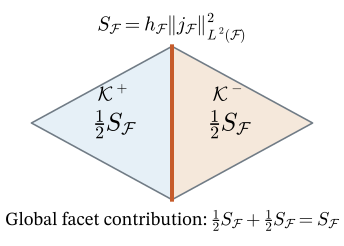
The indicators in Theorem 8.1 divide the squared estimator among individual elements. To see how their contributions combine, sum Equation 8.22 over all elements. Each interior facet appears twice, with a factor \(1/2\) each time; each Neumann facet appears once. Consequently,
\[ \eta^2 = \sum_{e=1}^{N_e}h_e^2\norm{r_e}_{L^2(\mathcal K_e)}^2 +\sum_{\mathcal F\in\mathcal F_h^{\mathrm{int}}\cup\mathcal F_h^{N}} h_{\mathcal F}\norm{j_{\mathcal F}}_{L^2(\mathcal F)}^2 . \tag{8.29}\]
The factor \(1/2\) allocates a shared contribution equally between its two neighbors (Arnold 2018, 73). The element-interior contribution remains entirely with its own element, as shown in Figure 8.6.
The upper-bound property Equation 8.24 is called reliability. The estimator uses only the mesh, \(u_h\), and the data \(f\), \(q\), and \(k\). In practice its integrals are evaluated by quadrature, which introduces a further approximation when the integrands are not integrated exactly.
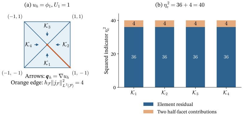
Example 8.3 (Computing the indicators on four triangles) Use \(P_1\) elements on the four-triangle mesh of Figure 8.7, with \(k=1\), \(f=3\), and \(u=0\) on the whole boundary. There is one free degree of freedom, at the center. Number the bottom, right, top, and left triangles \(\mathcal K_1,\ldots,\mathcal K_4\). The center basis function is
\[ \phi_1|_{\mathcal K_e}= \begin{cases} 1+x_2,&e=1,\\ 1-x_1,&e=2,\\ 1-x_2,&e=3,\\ 1+x_1,&e=4. \end{cases} \]
Each triangle has area one and diameter two. Its basis gradient has length one, and its integral of \(\phi_1\) is \(1/3\). Thus the single free equation is
\[ K_{11}U_1=F_1,\qquad K_{11}=\sum_{e=1}^4\int_{\mathcal K_e}|\grad\phi_1|^2\,\dx=4, \qquad F_1=3\sum_{e=1}^4\frac13=4. \]
Consequently \(U_1=1\) and \(u_h=\phi_1\). Its gradient is constant on each triangle, so \(r_e=3\). Consider the interior edge joining \((0,0)\) to \((1,-1)\). It separates the bottom triangle from the right triangle; take these as the plus and minus sides. The outward normal from the bottom triangle is \(\bn_{\mathcal F}=(1,1)^T/\sqrt2\). Substitution into Equation 8.13 gives
\[ j_{\mathcal F} =-\bigl((0,1)^T-(-1,0)^T\bigr)\cdot \frac{(1,1)^T}{\sqrt2}=-\sqrt2. \]
The edge has length \(h_{\mathcal F}=\sqrt2\), and hence
\[ h_{\mathcal F}\norm{j_{\mathcal F}}_{L^2(\mathcal F)}^2 =\sqrt2\int_{\mathcal F}2\,\ds=4. \]
The other three interior edges give the same contribution by symmetry. Every triangle shares two interior edges; its exterior edge is Dirichlet and contributes no facet term. Therefore
\[ \eta_e^2=2^2\int_{\mathcal K_e}3^2\,\dx +\frac12(4+4)=40, \qquad \eta^2=4\cdot40=160. \]
These nonzero indicators do not contradict the discrete equation. Indeed, \(\int_\Om3\phi_1\,\dx=4\), whereas on each interior edge \(\int_{\mathcal F}\phi_1\,\ds=\sqrt2/2\). The residual representation Equation 8.14 therefore gives \(R(u_h;\phi_1)=4+4(-\sqrt2)(\sqrt2/2)=0\). The signed terms cancel on this discrete test function, but their squared contributions to the estimator remain nonzero.
8.7 Marking elements and refining the mesh
The squared indicator \(\eta_e^2\) is the contribution assigned to an element in the sum \(\eta^2=\sum_e\eta_e^2\). It is not the exact squared error on that element. The bound Equation 8.24 controls the global error, not its exact distribution. We use the local contributions to choose where to refine, as follows.
8.7.1 Maximum and bulk marking
One simple choice is maximum marking. Given \(0<\rho<1\), mark
\[ \mathcal M=\{\mathcal K_e\in\Th: \eta_e\geq\rho\max_{e'}\eta_{e'}\}. \tag{8.30}\]
This selects elements relative to the largest indicator, without prescribing a fraction of the total squared estimator.
Dörfler marking, also called bulk marking, prescribes that fraction. Choose \(0<\theta<1\) and select a set \(\mathcal M\subset\Th\) satisfying
\[ \sum_{\mathcal K_e\in\mathcal M}\eta_e^2 \geq\theta\sum_{e=1}^{N_e}\eta_e^2=\theta\eta^2. \tag{8.31}\]
Sort the squared indicators in descending order and take the shortest initial portion whose sum reaches \(\theta\eta^2\). This gives a set of smallest cardinality satisfying the criterion; ties can give several such sets. A larger \(\theta\) selects at least as many elements in this procedure. Here \(\theta\) is the fraction of the squared estimator, not of \(\eta\) (Arnold 2018, 73).
Example 8.4 (Selecting contributions to the estimator) Suppose four squared indicators are \((16,9,4,1)\). Their sum is \(30\). For \(\theta=0.5\), the target is \(15\), so the first element alone is marked. For \(\theta=0.8\), the target is \(24\); the first two contributions total \(25\), so two elements are marked. Neither choice means that the marked elements contain exactly \(50\%\) or \(80\%\) of the true squared error.
8.7.2 Conforming refinement
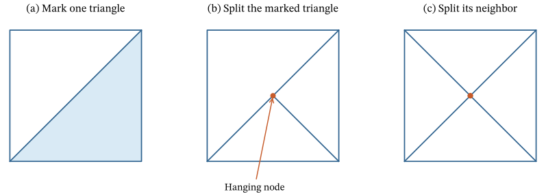
Refining a triangle inserts vertices and replaces it by smaller triangles. If an edge is split on only one side, its midpoint lies inside an edge of the neighboring triangle. Such a point is a hanging node. The ordinary continuous Lagrange space of Chapter 6 assumes a conforming mesh, so the neighbor must also be subdivided compatibly. Additional refinement needed to restore conformity is called mesh closure.
A refinement procedure must split the marked elements, restore conformity, and retain shape regularity. Repeated arbitrary subdivisions can produce increasingly flat triangles, invalidating uniform constants in the estimates. Standard bisection procedures are designed to avoid this problem (Larson and Bengzon 2010, sec. 4.9.2, pp. 89–90). The marked set is a request for refinement; the final refined region may be larger.
For fixed polynomial degree, conforming subdivision without changing the domain or boundary conditions gives nested spaces \(\Vhzero\subset\mathcal V_{h',0}\), where \(h'\) denotes the refined mesh. For the two Galerkin solutions, fine-mesh orthogonality gives \(a(u-u_{h'},u_{h'}-u_h)=0\). Expanding \(u-u_h=(u-u_{h'})+(u_{h'}-u_h)\) in the energy inner product yields
\[ \norm{u-u_h}_a^2 =\norm{u-u_{h'}}_a^2+\norm{u_{h'}-u_h}_a^2. \tag{8.32}\]
The energy error cannot increase under these assumptions. This does not say that each refinement reduces it by a prescribed factor, or that the computed estimator decreases at every step.
Exercise 8.3 (Comparing marking rules) Let \((\eta_1^2,\ldots,\eta_5^2)=(25,16,9,4,1)\).
- Find the marked elements for maximum marking with \(\rho=0.7\).
- Find a smallest bulk-marked set for \(\theta=0.7\).
- Compute the selected fraction of \(\eta^2\) in each case. Explain why the two parameters cannot be interpreted in the same way.
8.8 The adaptive finite element procedure
An adaptive computation repeats the following operations on a sequence of meshes \(\mathcal T_0,\mathcal T_1,\ldots\). The subscript counts adaptive cycles; it does not denote a uniform element size.
- Solve. Build the finite element space on the current mesh, impose boundary values, and solve for \(u_h\).
- Estimate. Compute every \(\eta_e^2\) and their sum \(\eta^2\).
- Check stopping. Stop if the estimator meets the chosen tolerance or the element, degree-of-freedom, or time budget is reached.
- Mark. Select \(\mathcal M\) by Equation 8.31.
- Refine. Refine \(\mathcal M\), restore conformity, and return to Step 1.
The solve step is essential after every refinement. Evaluating the old function on a finer mesh does not produce the new Galerkin solution. The spaces, forms, boundary data, and residuals must all refer to the current mesh.
8.8.1 Stopping and comparing computations
An estimator tolerance \(\eta\leq\varepsilon_{\mathrm{est}}\) implies
\[ \norm{u-u_h}_a\leq C_{\mathrm{rel}}\varepsilon_{\mathrm{est}}. \tag{8.33}\]
Because \(C_{\mathrm{rel}}\) is normally unknown numerically, this is not the certified assertion \(\norm{u-u_h}_a\leq\varepsilon_{\mathrm{est}}\). If the computation stops at a resource limit first, report that fact and the last estimator value.
A small change in an output, such as displacement at a point, does not establish a small global energy error. Likewise, a small energy error does not directly bound pointwise stress. The stopping quantity must match the accuracy being requested. Algebraic and quadrature errors should also be small enough not to dominate the discretization error being estimated.
On a nonuniform mesh, \(h=\max_e h_e\) can remain almost unchanged while the error decreases substantially. Compare uniform and adaptive refinement using error or estimator versus the number of degrees of freedom. Use the same counting convention for both sequences. The examples below count all scalar finite element degrees of freedom, including prescribed boundary values.
8.8.2 A refinement calculation in one dimension
The following example follows one complete marking and refinement step on a nonuniform bar mesh, for which the exact error can also be calculated.
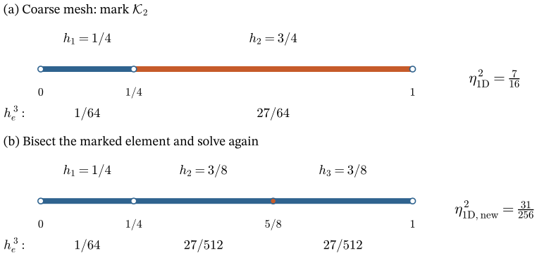
Example 8.5 (One refinement step for a bar) Take \(-u''=1\) on \((0,1)\) with \(u(0)=0\), \(u'(1)=0\), and nodes \((0,\tfrac14,1)\), as shown in Figure 8.9. As in Example 8.1, \(u=x-x^2/2\) and \(u_h=\Ih u\), with coefficients \((0,\tfrac7{32},\tfrac12)\). The slopes are \(7/8\) and \(3/8\), giving
\[ r_1=r_2=1,\qquad j_2=-\frac12,\qquad j_3=-\frac38. \]
For this one-dimensional problem, the residual estimate simplifies to
\[ \norm{u-u_h}_a\leq\eta_{\mathrm{1D}}, \qquad \eta_{\mathrm{1D}}^2 =\sum_{e=1}^{N_e}h_e^2\norm{r_e}_{L^2(\mathcal K_e)}^2 =\sum_{e=1}^{N_e}h_e^3. \tag{8.34}\]
The last equality uses \(r_e=1\). The one-dimensional bound uses nodal interpolation rather than quasi-interpolation; its facet terms vanish because the interpolation error is zero at every node (Larson and Bengzon 2010, 38–39). The contributions are \(1/64\) and \(27/64\), giving \(\eta_{\mathrm{1D}}^2=7/16\). Bulk marking with \(\theta=0.8\) selects the second element, which contributes \(27/28\) of the squared estimator.
Bisecting it gives lengths \((\tfrac14,\tfrac38,\tfrac38)\). After solving again,
\[ \eta_{\mathrm{1D,new}}^2 =\left(\frac14\right)^3+2\left(\frac38\right)^3 =\frac{31}{256}. \]
For this quadratic exact solution, the absolute derivative error on an element is the distance from its midpoint, so \(\norm{e}_a^2=\sum_e h_e^3/12\). The energy error decreases from \(\sqrt{7/192}\) to \(\sqrt{31/3072}\). This is a computed reduction, not an assumed reduction factor.
The nodal residuals remain part of the exact residual representation. They disappear only in the one-dimensional proof that tests with \(e-\Ih e\), which is zero at every node. In higher dimensions the facet terms must be retained.
Exercise 8.4 (The estimator for quadratic bar elements) Consider the uniformly loaded bar of Example 8.1 with quadratic elements.
- Use Example 5.6 to determine \(u_h\), and compute every element and facet residual.
- Explain why all residuals vanish. Use the one-dimensional residual representation in Example 8.1 and \(R(u_h;u-u_h)=\norm{u-u_h}_a^2\) to conclude that \(u_h=u\).
- Replace the load by \(f(x)=x\). Without solving, explain why the element residual of a quadratic approximation cannot vanish identically on every element. Identify the term in \(r_e\) that prevents this.
8.9 Implementing the estimator in FEniCSx
The companion adaptive-refinement notebook implements the complete procedure. It uses continuous \(P_1\) elements on triangles, \(k=1\), and homogeneous Dirichlet conditions on the whole boundary. There are no Neumann facets in its two examples. The notebook runs on one MPI process. The excerpts here explain indicator assembly; the notebook contains the solver, plotting, and refinement loop.
8.9.1 Storing one indicator per element
A degree-zero discontinuous space contains functions that are constant on each element, independently of neighboring elements. Denote it by
\[ W_h=\{z_h:z_h|_{\mathcal K_e}\text{ is constant for each }e\}. \]
Let \(\psi_e\) equal one on \(\mathcal K_e\) and zero on every other element. Assembling a linear functional on these test functions gives one vector entry per element. For example,
\[ B_{\mathrm{vol}}(\psi_e) =\sum_{e'}\int_{\mathcal K_{e'}}h_{e'}^2r_{e'}^2\psi_e\,\dx =h_e^2\norm{r_e}_{L^2(\mathcal K_e)}^2. \tag{8.35}\]
On an interior facet, use the average \((z_h^++z_h^-)/2\). Define
\[ B_{\mathrm{facet}}(z_h)= \sum_{\mathcal F\in\mathcal F_h^{\mathrm{int}}} \int_{\mathcal F}h_{\mathcal F}j_{\mathcal F}^2 \frac{z_h^++z_h^-}{2}\,\ds. \tag{8.36}\]
For \(z_h=\psi_e\), this assigns half of each adjacent interior-facet contribution to element \(e\). The assembled entry \(B_{\mathrm{vol}}(\psi_e)+B_{\mathrm{facet}}(\psi_e)\) is precisely \(\eta_e^2\). It is an integral contribution, not an element average; do not divide it by the element area.
The PDE solution space is still continuous. Using discontinuous constants to store indicators does not make it a discontinuous Galerkin method. A continuous piecewise-linear solution can have discontinuous gradients and therefore nonzero flux jumps.
8.9.2 Forms, vector entries, and refinement
With domain, u_h, and the UFL source f defined on the current mesh, the notebook writes
W = fem.functionspace(domain, ("DG", 0))
z = ufl.TestFunction(W)
h = ufl.CellDiameter(domain)
h_F = ufl.avg(ufl.FacetArea(domain))
n = ufl.FacetNormal(domain)

r = f + ufl.div(ufl.grad(u_h))
j = -ufl.jump(ufl.grad(u_h), n)

dx = ufl.Measure("dx", domain=domain,
                 metadata={"quadrature_degree": 20})
volume_form = h**2 * r**2 * z * dx
facet_form = (
    0.5 * h_F * j**2 * z("+") * ufl.dS
    + 0.5 * h_F * j**2 * z("-") * ufl.dS
)
dx integrates over element interiors and dS over interior facets. The restrictions ("+") and ("-") select the neighboring elements. jump(grad(u_h), n) is the sum of the two outward normal derivatives; its negative agrees with Equation 8.13. On a straight triangular mesh, FacetArea gives the edge length. Its two restrictions agree, so their average is \(h_{\mathcal F}\). In three dimensions, facet area is not facet diameter: this expression for the weight is specific to the two-dimensional notebook.
Assemble the forms separately and use the DG0 degree-of-freedom map to read the entry belonging to each element:
volume_vector = fem.assemble_vector(fem.form(volume_form))
facet_vector = fem.assemble_vector(fem.form(facet_form))
N_e = domain.topology.index_map(2).size_local
eta_squared = np.zeros(N_e)
for e in range(N_e):
    dof = W.dofmap.cell_dofs(e)[0]
    eta_squared[e] = (
        volume_vector.array[dof].real + facet_vector.array[dof].real
    )
eta = np.sqrt(np.sum(eta_squared))
Theory numbers elements from one; Python indices start at zero. The API name cell_dofs refers to element degrees of freedom. Dimension 2 denotes triangles. These arrays and sums suffice on the notebook’s single process; distributed assembly also requires communication and global sums.
Bulk marking is a short loop:
order = np.argsort(eta_squared)[::-1]
target = theta * eta_squared.sum()
marked = []
total = 0.0
for e in order:
    if total >= target:
        break
    marked.append(e)
    total += eta_squared[e]
The refinement call takes edge indices. Convert the marked triangle indices to a NumPy integer array and find their incident edges:
marked = np.asarray(marked, dtype=np.int32)
domain.topology.create_connectivity(2, 1)
edges = mesh.compute_incident_entities(domain.topology, marked, 2, 1)
refined_domain, _, _ = mesh.refine(domain, edges)
Dimensions 2 and 1 identify triangles and edges, respectively. The refinement routine also returns parent-entity information, which is unused here. Rebuild the space and coordinate-dependent data on refined_domain, solve again, and recompute the indicators.
Exercise 8.5 (Checking the half-facet contribution) Two triangles share one interior edge. Their volume residuals are zero and \(h_{\mathcal F}\norm{j_{\mathcal F}}_{L^2(\mathcal F)}^2=8\). Evaluate Equation 8.36 for each DG0 basis function. Find both squared indicators and the global estimator. What global value would result if both factors \(1/2\) in the code were omitted?
8.10 Adaptive computations
When the exact solution is known, we also report the effectivity index,
\[ I_{\mathrm{eff}}=\frac{\eta}{\norm{u-u_h}_a}, \qquad u_h\ne u. \tag{8.37}\]
A value near one means that the estimator closely approximates the error. Reliability only gives \(I_{\mathrm{eff}}\geq1/C_{\mathrm{rel}}\); it does not require this ratio to approach one.
8.10.1 A localized solution with a known error
Consider
\[ \left\{\begin{aligned} -\Delta u&=f&&\text{in }\Om=(0,1)^2,\\ u&=0&&\text{on }\partial\Om. \end{aligned}\right. \tag{8.38}\]
To concentrate the solution near the center, choose \(\beta=400\), set \(s_i=x_i-\tfrac12\), \(G_i=\exp(-\beta s_i^2)\), and \(c=\exp(-\beta/4)\). Prescribe
\[ u_{\mathrm{ex}}(x_1,x_2)=(G_1-c)(G_2-c). \tag{8.39}\]
At every boundary point at least one \(G_i=c\), so the boundary value is exactly zero. Differentiation gives the source
\[ \begin{aligned} f(x_1,x_2)=2\beta\bigl[ &(1-2\beta s_1^2)G_1(G_2-c)\\ &+(1-2\beta s_2^2)G_2(G_1-c)\bigr]. \end{aligned} \tag{8.40}\]
This follows the localized Gaussian example of Larson and Bengzon (2010, sec. 4.9.3, Eq. (4.130), p. 91), with a normalized amplitude and a boundary correction. The notebook calls the pulse parameter alpha; \(\beta\) here distinguishes it from the coercivity constant \(\alpha\).
Because the solution is known, compute
\[ E_a=\left(\int_\Om \grad(u_{\mathrm{ex}}-u_h)\cdot\grad(u_{\mathrm{ex}}-u_h)\,\dx\right)^{1/2}, \qquad I_{\mathrm{eff}}=\eta/E_a. \tag{8.41}\]
Use the analytic function in this error integral, not its nodal interpolant. The pulse and source are not polynomials. The notebook uses degree-20 volume quadrature; increasing it to degree 24 on the initial mesh changes \(\eta\) and \(E_a\) by relative amounts below \(4\times10^{-7}\). Quadrature must resolve the pulse before error comparisons are meaningful.
Start with \(8\times8\) squares, each divided into two triangles: 128 elements and 81 scalar degrees of freedom. Set \(\theta=0.5\). Initially, \(\eta\approx12.844\) and \(E_a\approx1.3233\). The first marked set has three elements and accounts for about \(60.7\%\) of \(\eta^2\): the selected sum exceeds the target because elements are selected whole. After refinement and a new solve, \(\eta\approx6.9622\) and \(E_a\approx0.76052\).
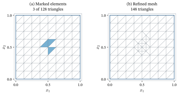
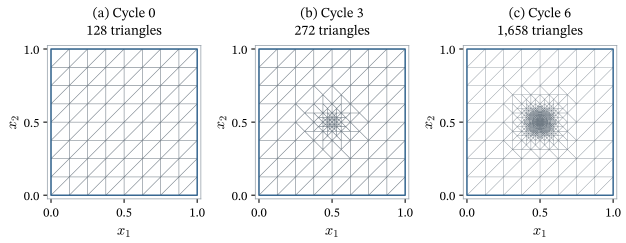
Figure 8.12 compares actual error and estimator against the total scalar degrees of freedom. At 2,869 degrees of freedom the adaptive error is about \(0.0831\); uniform refinement gives errors about \(0.3299\) at 4,225 degrees of freedom and \(0.1661\) at 16,641. For this localized solution, selective refinement reduces the measured error with far fewer unknowns.
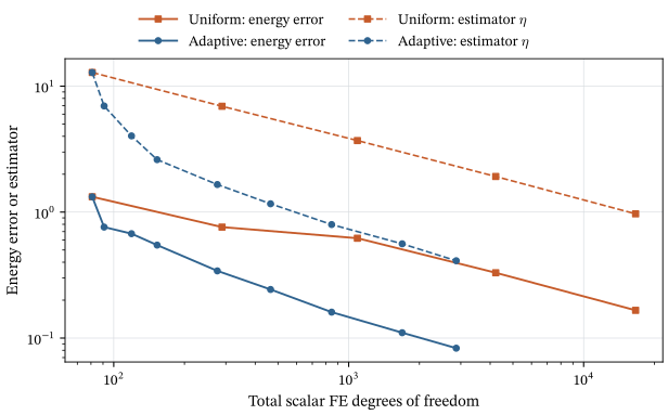
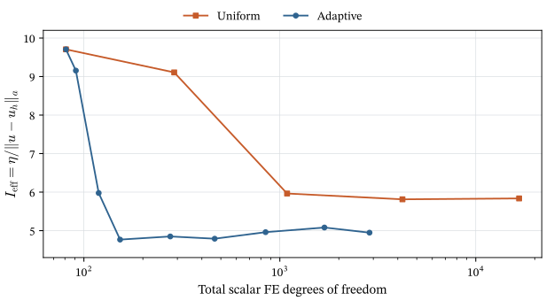
In Figure 8.13, adaptive effectivity approaches a factor near five, not one. This experiment does not determine the reliability constant for other data. The effect of unresolved variation in source data is discussed in Section 8.11.1.
8.10.2 A domain with a reentrant corner
Consider the L-shaped domain
\[ \Om=\{(x_1,x_2)\in(-1,1)^2:x_1<0\text{ or }x_2>0\}, \]
and solve
\[ \left\{\begin{aligned} -\Delta u&=1&&\text{in }\Om,\\ u&=0&&\text{on }\partial\Om. \end{aligned}\right. \tag{8.42}\]
The corner at \((0,0)\) has an interior angle greater than \(\pi\). The leading singular term has radial behavior \(r^{2/3}\), so this solution does not belong to \(H^2(\Om)\) (Arnold 2018, sec. 9.5, p. 74). The smooth-solution first-order energy estimate of Chapter 7 cannot be invoked on a uniform mesh. The reliability argument here needs the energy-space solution and the stated mesh and quasi-interpolation properties, not \(H^2\) regularity.
For \(P_1\) elements, \(r_e=1\). Although the source is constant, the indicators vary with element sizes and flux jumps. Starting from 24 triangles, the notebook performs seven solves and six refinements with \(\theta=0.5\). The estimator decreases from about \(1.3943\) to \(0.1782\).
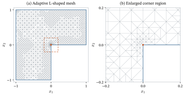
The exact solution is unavailable in this computation, so neither true error nor effectivity is reported. The mesh and estimator show where the method places resolution and how the computed estimate changes. They do not independently establish an exact convergence rate or a particular improvement over uniform refinement.
Exercise 8.6 (Verifying an adaptive calculation) Use the companion notebook for Equation 8.38.
- Change \(\theta\) to \(0.3\) and \(0.7\). Compare energy errors at comparable degree-of-freedom counts, not just at equal cycle numbers.
- On the initial mesh, sum the stored squared indicators and check that the marked elements satisfy Equation 8.31.
- Increase quadrature degree on the first two meshes and report relative changes in \(E_a\) and \(\eta\). Explain why this check is distinct from refining the finite element mesh.
8.11 Additional considerations
The residual estimate, indicator calculation, and adaptive procedure above form the main development of this chapter. The following considerations clarify the quality of an estimator and the scope of the argument.
8.11.1 Efficiency and data oscillation
Reliability bounds the error above by \(C_{\mathrm{rel}}\eta\). For refinement, we also want a large indicator to reflect a large error nearby rather than an unnecessarily large estimate. This is the purpose of a local efficiency bound. With the patch energy seminorm
\[ \norm{v}_{a,\omega_e} =\left(\int_{\omega_e}k|\grad v|^2\,\dx\right)^{1/2}, \]
the bound has the form
\[ \eta_e\leq C_{\mathrm{eff}} \bigl(\norm{u-u_h}_{a,\omega_e}+\mathrm{osc}_e\bigr). \tag{8.43}\]
The constant is independent of mesh size. The extra term \(\mathrm{osc}_e\) measures variation in the data that local polynomial approximations do not resolve. For unit-coefficient Poisson problems with \(P_1\) elements, use
\[ \overline f_e=\frac{1}{|\mathcal K_e|}\int_{\mathcal K_e}f\,\dx, \qquad \mathrm{osc}_e^2=\sum_{\mathcal K_{e'}\subset\omega_e} h_{e'}^2\norm{f-\overline f_{e'}}_{L^2(\mathcal K_{e'})}^2. \tag{8.44}\]
This term is zero for an elementwise-constant source. It is distinct from quadrature error and can be nonzero even when integrals are evaluated exactly. For \(k=1\), \(\Gam_D=\partial\Om\), and \(P_1\) elements on a conforming, shape-regular simplicial mesh, Equation 8.43 holds with this oscillation term. Its proof uses test functions supported on one element or on two elements sharing a facet; see Nochetto and Veeser (n.d., sec. 3.1, pp. 36–41, Theorem 7). We do not develop that separate proof here.
Together, reliability and efficiency relate the estimator to the error, up to constants and data oscillation. They do not make the estimator an exact error value. The effectivity index Equation 8.37 measures that numerical ratio when the exact solution is known. Neither the scalar reliability theorem nor the efficiency result just stated establishes coefficient-contrast-independent bounds for general discontinuous materials.
8.11.2 Linear elasticity
For the linear-elastic problem of Chapter 4, the computed stress is \(\bsig_h=\mathbb C:\beps(\bu_h)\). If it is smooth on each element, the same elementwise integration by parts gives the vector residuals
\[ \begin{aligned} \bm r_e&=\rho\bb+\divg\bsig_h,\\ \bm j_{\mathcal F}&=\begin{cases} -(\bsig_h^+\bn_{\mathcal F}-\bsig_h^-\bn_{\mathcal F}), &\mathcal F\in\mathcal F_h^{\mathrm{int}},\\ \overline{\bt}-\bsig_h\bn,&\mathcal F\in\mathcal F_h^N. \end{cases} \end{aligned} \tag{8.45}\]
Here \(\rho\bb\) and \(\overline{\bt}\) are the body force per unit volume and prescribed traction, and the boundary partition uses \(\Gam_D=\Gam_u\) and \(\Gam_N=\Gam_t\). The residuals measure force imbalance within elements, traction jumps between them, and mismatch with prescribed traction. Replacing the scalar residuals in Equation 8.22 by these vector residuals gives the corresponding estimator. Its analysis uses the elasticity energy norm \(\norm{\bv}_{a_{\mathrm{el}}}=\sqrt{a_{\mathrm{el}}(\bv,\bv)}\) and Korn’s inequality from Chapter 4. The scalar reliability constant cannot be reused unchanged.
Example 8.6 (Concentrated and distributed loading of a cantilever) Persistent refinement can reflect the loading model rather than an unresolved finite-energy solution. Consider the plane-stress cantilever \(\Om=(0,4)\times(0,1)\), fixed on \(x_1=0\), with no body force. Use unit thickness and consistent nondimensional data \(E=1\), \(\nu=0.3\), and \(P=10^{-6}\). The constitutive law is
\[ \bsig(\bu)=2\mu\beps(\bu) +\lambda_{\mathrm{ps}}\operatorname{tr}\beps(\bu)\bm I, \qquad \mu=\frac{E}{2(1+\nu)},\quad \lambda_{\mathrm{ps}}=\frac{E\nu}{1-\nu^2}. \]
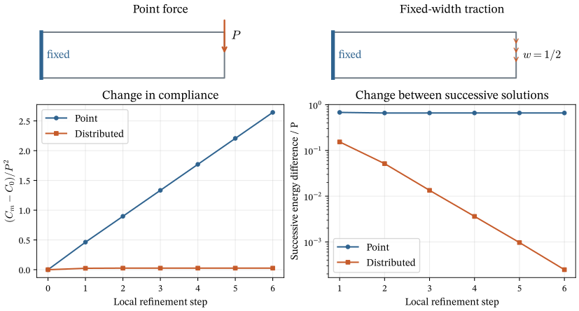
Compare a downward point force at \(\bx_P=(4,1/2)^T\) with a distributed traction on \(\Gam_P=\{4\}\times[1/4,3/4]\). For the latter, set \(w=1/2\), \(s=(x_2-1/4)/w\), and \(\overline{\bt}=(0,-6Ps(1-s)/w)^T\) on \(\Gam_P\), with zero traction elsewhere on the unfixed boundary. Both loads have downward resultant \(P\) and the same moment about the clamp. Their discrete load functionals are
\[ \ell_{\mathrm{point}}(\bv_h)=-P v_{h,2}(\bx_P), \qquad \ell_{\mathrm{dist}}(\bv_h) =\int_{\Gam_P}\overline{\bt}\cdot\bv_h\,\ds. \]
Use continuous vector-valued \(P_1\) elements with \(\bx_P\) a mesh node. The point force contributes \(-P\) to that node’s vertical load-vector entry; it is not a traction spread over a shrinking edge. The comparison notebook starts with \(64\times16\) rectangles split into triangles and repeatedly refines near \(\bx_P\), keeping the traction width fixed. This is prescribed local refinement, not residual-based marking.
Let \(\bu_m\) denote the solution after step \(m\) and define its compliance \(C_m=\ell(\bu_m)=a_{\mathrm{el}}(\bu_m,\bu_m)\); stored elastic energy is \(C_m/2\). For either fixed loading, nested spaces give \(a_{\mathrm{el}}(\bu_{m+1},\bu_m)=\ell(\bu_m)=C_m\). Expanding the squared energy norm gives
\[ \norm{\bu_{m+1}-\bu_m}_{a_{\mathrm{el}}}^2 =C_{m+1}-C_m. \tag{8.46}\]
In Figure 8.15, the point-load difference divided by \(P\) stays near \(0.661\), whereas the distributed-load difference falls from \(0.154\) to approximately \(0.000247\). The point-load compliance continues increasing by about \(0.436P^2\) per step. Displacement away from the load can nevertheless look settled: under uniform refinement, the two models give almost identical displacement at \((3,1/2)\).
Point evaluation is not bounded on the two-dimensional \(H^1\) energy space. The ideal point force therefore falls outside the finite-energy load assumptions used here, although every discrete system is solvable. The fixed-width traction is admissible. Refinement resolves the point-load singularity; it does not remove it. The computed differences are not true errors, and the ordinary \(L^2\) Neumann-residual term cannot be used for a Dirac force. These observations concern a two-dimensional continuum, not a point load in one-dimensional bar or beam theory.
8.11.3 Error in a linear output
Sometimes the requested output is a continuous linear functional \(G:\Vzero\to\R\), rather than the global energy norm. For example, \(G(v)=|D|^{-1}\int_Dv\,\dx\) is the average over a fixed subdomain \(D\subset\Om\) of positive volume. Define the dual solution \(z\in\Vzero\) by
\[ a(v,z)=G(v)\qquad\forall v\in\Vzero. \tag{8.47}\]
With \(e=u-u_h\), choose \(v=e\) in this equation and use Equation 8.3 with test function \(z\). For any \(z_h\in\Vhzero\), Galerkin orthogonality gives
\[ G(u)-G(u_h)=G(e)=a(e,z)=R(u_h;z)=R(u_h;z-z_h). \tag{8.48}\]
The residual is weighted by the dual error: its contribution depends on its effect on the requested output. This is the goal-oriented use of duality anticipated in Chapter 7. The identity is exact but not computable as written, because \(z\) is unknown. Directly testing with a dual approximation in the same discrete space gives zero by Galerkin orthogonality. A practical dual-weighted residual method requires an enriched dual approximation or an appropriate reconstruction. Developing and analyzing that estimator is outside this chapter’s energy-error treatment.
8.12 Chapter summary
The residual \(R(u_h;v)=\ell(v)-a(u_h,v)\) relates the computed solution to the error through \(R(u_h;v)=a(u-u_h,v)\). Its energy dual norm equals the energy error exactly, but that supremum is not directly computable.
Elementwise integration by parts separates the residual into \(r_e=f+\divg(k\grad u_h)\), interior normal-flux jumps, and Neumann mismatches. Their weighted squared norms define the indicators.
Galerkin orthogonality permits testing with \(e-\mathcal Q_he\). Local approximation estimates and finite patch overlap give \(\norm{u-u_h}_a\leq C_{\mathrm{rel}}\eta\). The quasi-interpolation estimates are assumed explicitly for the general mixed-boundary setting.
Local efficiency relates an indicator to nearby error and data oscillation; this additional property is stated for unit-coefficient, fully Dirichlet Poisson problems with linear elements. Effectivity measures the estimator’s ratio to the actual error, not the computational cost.
The squared indicators distribute \(\eta^2\) among elements. Bulk marking selects a prescribed fraction of that sum, and conforming refinement produces the next mesh. Solving again completes one adaptive cycle.
The Gaussian example verifies the estimator against an analytic solution; the corner example uses the same procedure without assuming a smooth or known exact solution. In the latter case, the estimator is available but the true error and effectivity are not.