import numpy as np

mu, lam, tau = 1.0, 2.0, 1.0
L0, A0 = 1.0, 1.0
x = np.linspace(0.0, L0, 3)
U = np.zeros(len(x))
free = np.arange(1, len(x))
F_load = np.zeros(len(x))
F_load[-1] = A0 * tau

def assemble(U):
    R = F_load.copy()
    K_T = np.zeros((len(x), len(x)))
    for e in range(len(x) - 1):
        ids = [e, e + 1]
        Le = x[e + 1] - x[e]
        s = 1 + (U[e + 1] - U[e]) / Le
        if s <= 0:
            raise ValueError("Nonpositive element stretch")
        P = mu * (s - 1/s) + lam * np.log(s)/s
        dP = mu * (1 + 1/s**2) + lam * (1 - np.log(s))/s**2
        f_int = A0 * P * np.array([-1.0, 1.0])
        K_e = -A0 * dP/Le * np.array([[1.0, -1.0], [-1.0, 1.0]])
        for a in range(2):
            R[ids[a]] -= f_int[a]
            for b in range(2):
                K_T[ids[a], ids[b]] += K_e[a, b]
    return R, K_T

for k in range(20):
    R, K_T = assemble(U)
    if np.linalg.norm(R[free]) < 1e-9:
        break
    delta_U = np.linalg.solve(K_T[np.ix_(free, free)], -R[free])
    U[free] += delta_U
else:
    raise RuntimeError("Newton iteration did not converge")

reaction = -R[0]
print("U =", U)
print("Support reaction =", reaction)9 Nonlinear Finite Element Methods
The linear problems of Chapters 5 and 6 led to a matrix equation \(\bK\bU=\bF\). Once the mesh, material parameters, and boundary data were specified, the matrix did not depend on the unknown displacement. Finite deformation changes this situation. In the hyperelastic problem of Section 4.5, the stress depends on \(\bF(\bu)=\bI+\Grad\bu\) through its determinant and inverse. Substituting a finite element displacement into the variational equation therefore gives nonlinear equations for its coefficients.
This chapter develops Newton’s method for those equations. We can linearize the variational residual and then discretize the correction equation, or discretize the nonlinear problem and then differentiate its algebraic residual. Both routes give the same Newton system under the conditions stated in Section 9.4.4. After the full Newton iteration, we consider two ways to help it converge: load stepping gives a starting displacement for the next load, and a line search can shorten a correction at a fixed load. The final example applies the same formulation to a scalar nonlinear diffusion problem.
9.1 Equilibrium, residual, and energy
9.1.1 The reference-configuration problem
Let \(\Om_0\subset\R^3\) be the reference body, with prescribed displacement \(\overline{\bu}\) on \(\Gam_{0u}\) and prescribed reference traction \(\overline{\bt}_0\) on \(\Gam_{0t}\). The body force \(\bb_0\) is measured per unit reference volume. Throughout the chapter, these loads are independent of displacement. The reference geometry remains fixed while the current configuration is determined by \(\bx=\bX+\bu(\bX)\).
Recall the strong problem Equation 4.64 and the spaces Equation 4.70:
\[ \begin{aligned} \mathcal U_{\overline{\bu}} &=\{\bw\in H^1(\Om_0;\R^3):\bw=\overline{\bu} \text{ on }\Gam_{0u}\},\\ \Vzero &=\{\bv\in H^1(\Om_0;\R^3):\bv=\bm0 \text{ on }\Gam_{0u}\}. \end{aligned} \tag{9.1}\]
As in Remark 4.6, we assume enough regularity for the following stress and energy integrals to be finite. Deformations must satisfy \(J=\det\bF>0\); the \(H^1\) condition alone does not impose this requirement. Our purpose here is the construction and solution of the discrete equations, not an existence theory for nonlinear elasticity.
The internal and external forms from Equation 4.74 are
\[ \begin{aligned} a_{\mathrm{hyp}}(\bu;\bv) &=\int_{\Om_0}\bP(\bF(\bu)):\Grad\bv\,\dd V,\\ \ell_{\mathrm{hyp}}(\bv) &=\int_{\Om_0}\bb_0\cdot\bv\,\dd V +\int_{\Gam_{0t}}\overline{\bt}_0\cdot\bv\,\dd A. \end{aligned} \tag{9.2}\]
The first is generally nonlinear in \(\bu\) and linear in \(\bv\); the second is linear in \(\bv\). Define their residual using external minus internal work:
\[ R(\bu;\bv)=\ell_{\mathrm{hyp}}(\bv)-a_{\mathrm{hyp}}(\bu;\bv). \tag{9.3}\]
The nonlinear variational problem is
\[ \boxed{\text{Find }\bu\in\mathcal U_{\overline{\bu}}\text{ such that } R(\bu;\bv)=0\quad\forall\bv\in\Vzero.} \tag{9.4}\]
A trial displacement satisfies the prescribed boundary displacement but need not satisfy Equation 9.4. Its nonzero residual supplies the right-hand side for a correction.
9.1.2 First and second variations of the potential
For the displacement-independent loads in Equation 9.2, the total potential from Equation 4.77 can be written
\[ \Pi_{\mathrm{hyp}}(\bu) =\int_{\Om_0}\Psi(\bF(\bu))\,\dd V-\ell_{\mathrm{hyp}}(\bu). \tag{9.5}\]
For the variations below, assume sufficient regularity to differentiate under the integral and use directions for which the perturbed displacement remains admissible for sufficiently small \(|\epsilon|\). In particular, zero prescribed displacement of a direction alone does not guarantee that \(J\) stays positive along the perturbation.
The first variation was defined in Definition 2.25. Since \(\bF(\bu+\epsilon\bv)=\bF(\bu)+\epsilon\Grad\bv\) and \(\bP=\partial\Psi/\partial\bF\), the chain rule gives
\[ \begin{aligned} \delta\Pi_{\mathrm{hyp}}(\bu;\bv) &=\left.\frac{\dd}{\dd\epsilon} \Pi_{\mathrm{hyp}}(\bu+\epsilon\bv)\right|_{\epsilon=0}\\ &=\int_{\Om_0}\bP(\bF(\bu)):\Grad\bv\,\dd V -\ell_{\mathrm{hyp}}(\bv)\\ &=-R(\bu;\bv). \end{aligned} \tag{9.6}\]
Consequently, stationarity for every admissible direction \(\bv\) is exactly the variational equation Equation 9.4. This equivalence concerns stationary points; a stationary point need not minimize the potential.
Newton’s method requires the variation of the residual with respect to the displacement. Hold the test function \(\bv\) fixed and perturb \(\bu\) in a direction \(\bw\in\Vzero\):
\[ \delta_uR(\bu;\bv)[\bw] :=\left.\frac{\dd}{\dd\epsilon} R(\bu+\epsilon\bw;\bv)\right|_{\epsilon=0}. \tag{9.7}\]
For a twice-differentiable potential, its second variation is
\[ \delta^2\Pi_{\mathrm{hyp}}(\bu;\bv,\bw) :=\left.\frac{\dd}{\dd\epsilon} \delta\Pi_{\mathrm{hyp}}(\bu+\epsilon\bw;\bv)\right|_{\epsilon=0}. \tag{9.8}\]
Differentiating Equation 9.6 with \(\bv\) fixed gives
\[ \boxed{\delta_uR(\bu;\bv)[\bw] =-\delta^2\Pi_{\mathrm{hyp}}(\bu;\bv,\bw).} \tag{9.9}\]
Thus the residual derivative and the second variation describe the same linearized stress response, with opposite signs under our residual convention. If the second derivative is continuous, the second variation is symmetric in \(\bv\) and \(\bw\). Symmetry alone does not establish positivity or stability.
Exercise 9.1 (Energy and the residual of a nonlinear spring) Let \(\Pi(z)=kz^2/2+cz^4/4-Pz\), where \(k,c>0\) and \(P\) is prescribed. Define the residual as applied force minus spring force.
- Find \(r(z)\) and verify \(\delta\Pi(z;v)=-r(z)v\).
- Calculate \(\delta^2\Pi(z;v,w)\) and \(r'(z)vw\). Verify their sign relation.
- Show that \(\Pi''(z)>0\) for every \(z\), and explain why this particular spring has at most one equilibrium for a given \(P\).
9.2 Newton’s method
9.2.1 A scalar equation
Consider a scalar equation \(r(z)=0\), with \(r\) twice continuously differentiable near the iterate. Given an approximation \(z^k\), write the next approximation as \(z^{k+1}=z^k+\Delta z^k\). Taylor expansion gives
\[ r(z^k+\Delta z^k) =r(z^k)+r'(z^k)\Delta z^k+O((\Delta z^k)^2). \]
Newton’s method sets the first-order approximation to zero and solves
\[ \boxed{r'(z^k)\Delta z^k=-r(z^k), \qquad z^{k+1}=z^k+\Delta z^k.} \tag{9.10}\]
The correction requires \(r'(z^k)\ne 0\). Evaluate the derivative at the current approximation. Reusing a derivative from an earlier iterate defines a different iteration and need not give Newton’s convergence rate (Belytschko et al. 2000).
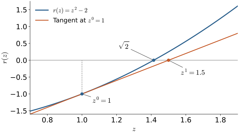
Example 9.1 (Computing a square root) For \(r(z)=z^2-2\), \(r'(z)=2z\). Starting from \(z^0=1\), the first correction is
\[ 2\Delta z^0=1,\qquad \Delta z^0=\frac12,\qquad z^1=1.5. \]
In general, Equation 9.10 becomes
\[ z^{k+1}=z^k-\frac{(z^k)^2-2}{2z^k} =\frac12\left(z^k+\frac2{z^k}\right). \]
| \(k\) | \(z^k\) | \(|r(z^k)|\) |
|---|---|---|
| 0 | 1.000000 | \(1\) |
| 1 | 1.500000 | \(0.25\) |
| 2 | 1.416667 | \(6.9444\times10^{-3}\) |
| 3 | 1.414216 | \(6.0073\times10^{-6}\) |
The iterates approach \(\sqrt2\). The tangent construction is shown in Figure 9.1. Starting instead at \(z^0=0\) would fail because the linear correction equation would have zero coefficient and nonzero right-hand side.
9.2.2 Correction of a displacement field
For Equation 9.4, the unknown is a field rather than a scalar. Keep \(\bv\in\Vzero\) fixed and expand the residual about \(\bu^k\):
\[ R(\bu^k+\Delta\bu^k;\bv) \approx R(\bu^k;\bv)+\delta_uR(\bu^k;\bv)[\Delta\bu^k]. \]
Setting this approximation to zero gives the formal Newton equation for the displacement field:
\[ \boxed{\begin{aligned} &\text{Find }\Delta\bu^k\in\Vzero\text{ such that}\\ &\delta_uR(\bu^k;\bv)[\Delta\bu^k] =-R(\bu^k;\bv)\quad\forall\bv\in\Vzero. \end{aligned}} \tag{9.11}\]
The coefficients depend on \(\bu^k\), but the equation is linear in \(\Delta\bu^k\). This derivation assumes that the residual can be differentiated in the directions used. The \(H^1\) boundary-value spaces and \(J>0\) alone do not ensure this: \(\bF^{-1}\) can become unbounded as \(J\) approaches zero. In Section 9.4 we solve the finite element version of Equation 9.11, then update the displacement and reevaluate the residual.
The zero boundary value of the correction follows from the boundary data, not from assuming that the prescribed displacement is zero. Suppose the initial iterate satisfies \(\bu^0=\overline{\bu}\) on \(\Gam_{0u}\) and that the data are fixed during this solve. At iteration \(k\),
\[ \begin{aligned} \bu^{k+1}=\bu^k+\Delta\bu^k&=\overline{\bu} &&\text{on }\Gam_{0u},\\ \Delta\bu^k&=\overline{\bu}-\bu^k=\bm0 &&\text{on }\Gam_{0u}. \end{aligned} \tag{9.12}\]
Thus every update preserves the prescribed displacement. Assigning \(\Delta\bu^k=\overline{\bu}\) instead would repeatedly add the boundary displacement and solve a different problem.
9.3 Consistent linearization of hyperelasticity
9.3.1 Differentiating the stress work
We now calculate the derivative in Equation 9.11. Since the loads in Equation 9.2 are independent of \(\bu\),
\[ \delta_uR(\bu;\bv)[\bw] =-\delta_u a_{\mathrm{hyp}}(\bu;\bv)[\bw]. \]
The perturbation of the deformation gradient is
\[ \bF(\bu+\epsilon\bw) =\bI+\Grad\bu+\epsilon\Grad\bw =\bF(\bu)+\epsilon\Grad\bw. \tag{9.13}\]
For a tensor direction \(\bm H\), define the stress variation by
\[ \delta\bP(\bF;\bm H) :=\left.\frac{\dd}{\dd\epsilon} \bP(\bF+\epsilon\bm H)\right|_{\epsilon=0}. \tag{9.14}\]
Substitute \(\bm H=\Grad\bw\) into Equation 9.14 and differentiate the internal-work integral. Assuming sufficient smoothness to differentiate under the integral,
\[ \boxed{\delta_uR(\bu;\bv)[\bw] =-\int_{\Om_0}\delta\bP(\bF(\bu);\Grad\bw):\Grad\bv\,\dd V.} \tag{9.15}\]
In particular, with \(\bF^k=\bI+\Grad\bu^k\), Equation 9.11 is
\[ -\int_{\Om_0}\delta\bP(\bF^k;\Grad\Delta\bu^k):\Grad\bv\,\dd V =-R(\bu^k;\bv)\quad\forall\bv\in\Vzero. \tag{9.16}\]
The minus sign on the integral comes from \(R=\ell-a\); the one on the right comes from moving the current residual to the right-hand side of Newton’s equation.
9.3.2 The neo-Hookean material tangent
For the stress law in Equation 4.69, the stress variation is
\[ \begin{aligned} \delta\bP(\bF;\bm H) ={}&\mu\bm H +\lambda\tr(\bF^{-1}\bm H)\bF^{-T}\\ &+(\mu-\lambda\ln J)\bF^{-T}\bm H^T\bF^{-T}. \end{aligned} \tag{9.17}\]
Appendix C derives this result by differentiating the inverse and determinant of \(\bF\). In the Newton equation, evaluate it at \(\bF^k\) and use \(\bm H=\Grad\Delta\bu^k\). This is a consistent tangent: it differentiates the stress law used to compute the residual. Using the small-strain stiffness with the finite-deformation residual would give a different correction equation.
Example 9.2 (Recovery of the linear elastic response) At the undeformed state, \(\bF=\bI\) and \(J=1\), Equation 9.17 becomes
\[ \delta\bP(\bI;\bm H) =\mu(\bm H+\bm H^T)+\lambda\tr(\bm H)\bI. \]
Set \(\bm H=\Grad\bw\). Since \(\beps(\bw)=(\Grad\bw+(\Grad\bw)^T)/2\), this is
\[ \delta\bP(\bI;\Grad\bw) =2\mu\beps(\bw)+\lambda\tr(\beps(\bw))\bI. \]
This is the isotropic linear elastic stress associated with the incremental displacement \(\bw\). The finite-deformation law therefore recovers the small-strain law at first order about its stress-free reference state.
Exercise 9.2 (A shear perturbation) At \(\bF=\bI\), let \(\bm H=\gamma\bm e_1\otimes\bm e_2\). Use Equation 9.17 to calculate every nonzero component of \(\delta\bP(\bI;\bm H)\). Repeat with the skew-symmetric direction \(\bm H=\gamma(\bm e_1\otimes\bm e_2-\bm e_2\otimes\bm e_1)\). Explain the second result using the infinitesimal strain of that direction.
9.4 Finite element residual and tangent matrix
9.4.1 Coefficients, free directions, and equilibrium equations
Use a conforming reference mesh \(\Th\) and scalar nodal basis functions \(\phi_i\), \(i=1,\ldots,N_n\). Following the vector-valued construction in Chapter 6, write
\[ \bu_h(\bX)=\sum_{i=1}^{N_n}\phi_i(\bX)\bm U_i, \qquad \bm U_i=\begin{bmatrix}U_{i1}&U_{i2}&U_{i3}\end{bmatrix}^{T}. \tag{9.18}\]
Stack the nodal vectors into \(\bU\). Here \(i,j\) label nodes and Greek indices \(\alpha,\beta\) label spatial components. A vector basis direction is \(\phi_i\bm e_\alpha\), where \(\bm e_\alpha\) is a Cartesian unit vector. The discrete test space \(\Vhzero\subset\Vzero\) consists of the finite element fields with zero prescribed displacement. Only free basis directions belong to this space. The discrete trial space satisfies the prescribed displacement, with coefficients denoted by \(\bU_p=\overline{\bU}_p\).
Define the load and residual entries before eliminating prescribed rows:
\[ \begin{aligned} F_{i\alpha}&=\ell_{\mathrm{hyp}}(\phi_i\bm e_\alpha),\\ R_{i\alpha}(\bU) &=F_{i\alpha}-\int_{\Om_0} \bP(\bF(\bu_h)):\Grad(\phi_i\bm e_\alpha)\,\dd V\\ &=R(\bu_h;\phi_i\bm e_\alpha). \end{aligned} \tag{9.19}\]
Thus the algebraic residual has exactly the sign of the variational residual. The discrete equilibrium equations are \(\bR_f(\bU)=\bm0\) on free rows. Prescribed rows define force imbalances, not equations that must vanish: the support reactions are \(\bm r_p=-\bR_p\) as in Equation 5.48. The components \(F_{i\alpha}\) are nodal loads, whereas \(F_{\alpha I}\) is a component of the deformation gradient, with \(I\) indexing the reference-coordinate directions.
9.4.2 Linearize, then discretize
Start with the linearized variational equation Equation 9.11. Evaluate it at the current FE displacement \(\bu_h^k\) and expand the correction:
\[ \Delta\bu_h^k=\sum_{j,\beta}\phi_j\bm e_\beta\Delta U_{j\beta}^k. \]
The prescribed correction coefficients in this expansion are zero by Equation 9.12. Choose \(\bv_h=\phi_i\bm e_\alpha\) for a free row. Linearity in the correction direction gives
\[ \sum_{j,\beta} \delta_uR(\bu_h^k;\phi_i\bm e_\alpha)[\phi_j\bm e_\beta] \Delta U_{j\beta}^k =-R(\bu_h^k;\phi_i\bm e_\alpha). \]
The coefficient of \(\Delta U_{j\beta}^k\) defines the tangent entry. Using Equation 9.15 with \(\bF^k=\bI+\Grad\bu_h^k\) gives
\[ \begin{aligned} (K_T)_{i\alpha,j\beta}(\bU^k) &=\delta_uR(\bu_h^k;\phi_i\bm e_\alpha)[\phi_j\bm e_\beta]\\ &=-\int_{\Om_0}\delta\bP(\bF^k;\Grad(\phi_j\bm e_\beta)) :\Grad(\phi_i\bm e_\alpha)\,\dd V. \end{aligned} \tag{9.20}\]
The right-hand side is minus the residual entry in Equation 9.19. Thus the free Newton rows are
\[ \sum_{j,\beta}(K_T)_{i\alpha,j\beta}(\bU^k)\Delta U_{j\beta}^k =-R_{i\alpha}(\bU^k). \tag{9.21}\]
The test direction determines the row, and the correction basis direction determines the column. This is the sequence used in Section 9.9: differentiate the variational form, then assemble the matrix.
9.4.3 Discretize, then linearize
In this route, substitute Equation 9.18 into the nonlinear variational problem and test with the free basis directions. This gives the nonlinear algebraic equations \(\bR_f(\bU)=\bm0\) from Equation 9.19. With the prescribed coefficients held fixed, Newton’s method now acts directly on those equations:
\[ \sum_{j,\beta\text{ free}} \frac{\partial R_{i\alpha}}{\partial U_{j\beta}}(\bU^k) \Delta U_{j\beta}^k=-R_{i\alpha}(\bU^k), \qquad i\alpha\text{ free}. \tag{9.22}\]
To compute one derivative, change only \(U_{j\beta}\) by \(\epsilon\). The finite element displacement then changes from \(\bu_h\) to \(\bu_h+\epsilon\phi_j\bm e_\beta\). The test direction does not change. Substituting the perturbed displacement into the definition of \(R_{i\alpha}\) gives
\[ \begin{aligned} \frac{\partial R_{i\alpha}}{\partial U_{j\beta}}(\bU) &=\left.\frac{\dd}{\dd\epsilon} R(\bu_h+\epsilon\phi_j\bm e_\beta;\phi_i\bm e_\alpha) \right|_{\epsilon=0}\\ &=\delta_u R(\bu_h;\phi_i\bm e_\alpha)[\phi_j\bm e_\beta] =(K_T)_{i\alpha,j\beta}(\bU). \end{aligned} \tag{9.23}\]
9.4.4 When the two routes give the same matrix
In Section 9.4.2, we differentiate with respect to a field, then evaluate the derivative on pairs of finite element basis directions. In Section 9.4.3, we differentiate with respect to the coefficients of those directions. By Equation 9.23, both give the same matrix. In an implementation, use the same spaces, prescribed coefficients, and quadrature in both routes. With fixed quadrature points and weights, differentiation of the discrete residual amounts to differentiating the same weighted sum of integrand values. An independently chosen quadrature rule for the tangent need not produce the Jacobian of that residual. For the displacement-independent loads here, \(R=\ell-a\) makes \(\bK_T\) the negative of the internal-force derivative.
In Section 9.9, UFL differentiates the residual form before DOLFINx assembles the matrix. Differentiating after discretization is useful when the residual is already available as an algebraic function of the coefficients. See also Arnold (2018, sec. 10.2) and Larson and Bengzon (2010, secs. 9.2–9.4).
9.4.5 The discrete potential
For a hyperelastic material, let \(\Pi_h(\bU)=\Pi_{\mathrm{hyp}}(\bu_h)\) be the discrete potential. Then Equation 9.6 evaluated on each free basis direction, with prescribed coefficients held fixed, shows that
\[ \bR_f=-\nabla_{\bU_f}\Pi_h, \qquad (K_T)_{ff}=-\nabla_{\bU_f}^{\,2}\Pi_h. \tag{9.24}\]
For a twice continuously differentiable \(\Pi_h\), this free Jacobian is symmetric. It need not be positive definite. At a strict local minimum with positive definite energy Hessian on free directions, \((K_T)_{ff}\) is negative definite.
9.4.6 Prescribed coefficients and reactions
Partition \(\bU\) into free and prescribed entries. If \(\bU_p^k=\overline{\bU}_p\), Equation 9.12 gives \(\Delta\bU_p^k=\bm0\). The free rows of Equation 9.21 are
\[ (K_T)_{ff}\Delta\bU_f^k +(K_T)_{fp}\underbrace{\Delta\bU_p^k}_{\bm0} =-\bR_f(\bU^k). \]
Thus the system actually solved is
\[ \boxed{(K_T)_{ff}(\bU^k)\Delta\bU_f^k=-\bR_f(\bU^k), \qquad \bU_f^{k+1}=\bU_f^k+\Delta\bU_f^k.} \tag{9.25}\]
Keep \(\bU_p^{k+1}=\overline{\bU}_p\). The residual and tangent are evaluated using the full displacement vector, including the prescribed values. Once the solve converges, assemble the full residual without replacing its prescribed rows by boundary equations. The support reactions are
\[ \bm r_p=-\bR_p(\bU). \tag{9.26}\]
These reactions are additional external forces supplied by the supports. They balance the applied forces when the free equations are satisfied.
9.5 Worked stretch problem and an explicit implementation
Example 9.3 (Homogeneous constrained stretch) Consider a prismatic body of reference length \(L_0\) and area \(A_0\). Constrain transverse displacement throughout the body and seek an axial displacement independent of transverse position. With no body force, the homogeneous deformation is
\[ \bu(\bX)=\begin{bmatrix}(s-1)X_1&0&0\end{bmatrix}^{T}, \qquad \bF=\operatorname{diag}(s,1,1),\qquad J=s>0. \]
The stretch \(s\) is dimensionless. Impose \(u_1=0\) at \(X_1=0\) and reference traction \(\tau\bm e_1\) on the end \(X_1=L_0\). This is a constrained stretch, not a bar with traction-free lateral contraction: the transverse constraints supply reactions. Substitution into Equation 4.69 gives
\[ P_{11}(s)=\mu(s-s^{-1})+\lambda\frac{\ln s}{s}. \tag{9.27}\]
The axial equilibrium equation and its derivative are
\[ \begin{aligned} r(s)&=\tau-P_{11}(s)=0,\\ r'(s)&=-\mu(1+s^{-2})-\lambda\frac{1-\ln s}{s^2}. \end{aligned} \tag{9.28}\]
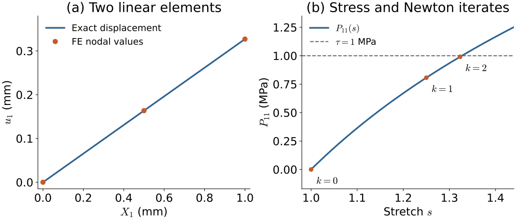
For \(\mu=1\) MPa, \(\lambda=2\) MPa, and \(\tau=1\) MPa, start at \(s^0=1\). The first Newton equation is \((-4\ \mathrm{MPa})\Delta s^0=-1\ \mathrm{MPa}\), giving \(s^1=1.25\). Recomputing \(r\) and \(r'\) after each update gives
| \(k\) | \(s^k\) | \(r(s^k)\) (MPa) | \(\Delta s^k\) |
|---|---|---|---|
| 0 | 1.000000 | \(1\) | \(0.250000\) |
| 1 | 1.250000 | \(0.192970\) | \(0.073251\) |
| 2 | 1.323251 | \(0.009125\) | \(0.003813\) |
| 3 | 1.327064 | \(2.1507\times10^{-5}\) | \(9.0286\times10^{-6}\) |
| 4 | 1.327073 | \(1.1978\times10^{-10}\) | — |
The computed stretch is approximately \(1.327072596\). The deformation remains admissible throughout this iteration.
9.5.1 Element equations for the constrained problem
We can assemble the finite element equations for this example by hand. Divide \([0,L_0]\) into linear elements. For element \(e\) of length \(L_e\), the local axial coefficients \(U_1^e,U_2^e\) give the stretch
\[ s_e=1+\frac{U_2^e-U_1^e}{L_e}. \]
The axial basis derivatives are \((-1/L_e,1/L_e)\). The stress is constant on the element, so its internal-force vector and residual derivative are
\[ \begin{aligned} \bm f_{\mathrm{int}}^e &=A_0P_{11}(s_e)\begin{bmatrix}-1\\1\end{bmatrix},\\ \bK_T^e &=-\frac{A_0P_{11}'(s_e)}{L_e} \begin{bmatrix}1&-1\\-1&1\end{bmatrix}. \end{aligned} \tag{9.29}\]
To check the sign, differentiate \(s_e=1+(U_2^e-U_1^e)/L_e\): its coefficient derivatives are \((-1/L_e,1/L_e)\). Differentiating \(-\bm f_{\mathrm{int}}^e\) with these derivatives produces the negative matrix in Equation 9.29. The only applied load is the end force \(A_0\tau\). Assemble \(\bR=\bF-\bm f_{\mathrm{int}}\) and impose \(U_1=0\).
Take two equal elements, with \(L_0=1\) mm and \(A_0=1\) mm\(^2\). At the initial displacement \(\bU^0=\bm0\), each element has \(s_e=1\), \(P_{11}(1)=0\), and \(P_{11}'(1)=4\) MPa. Thus the internal forces are zero and each element tangent is the matrix in Equation 9.29 with prefactor \(-8\) N/mm. Node 2 receives a diagonal contribution from both elements; node 3 receives one from the second element. The free residual is \(\bR_f(\bU^0)=(0,1)^T\) N because only node 3 carries the end load. Using Equation 9.25, with matrix entries in N/mm and forces in N, the first correction solves
\[ \begin{bmatrix}-16&8\\8&-8\end{bmatrix} \begin{bmatrix}\Delta U_2^0\\ \Delta U_3^0\end{bmatrix} =\begin{bmatrix}0\\-1\end{bmatrix}, \qquad \begin{bmatrix}\Delta U_2^0\\ \Delta U_3^0\end{bmatrix} =\begin{bmatrix}0.125\\0.25\end{bmatrix}\ \mathrm{mm}. \tag{9.30}\]
The next iterate is \(\bU^1=(0,0.125,0.25)^T\) mm. Both elements now have stretch \(1.25\), the first updated value in the scalar example. The program below repeats this calculation until the residual is small.
The following NumPy program uses millimeters, newtons, and megapascals, so \(L_0=A_0=1\) means \(1\) mm and \(1\) mm\(^2\), respectively. As in Chapters 5 and 6, Python uses zero-based indices. The arrays ids = [e, e + 1] implement the two-node connectivity; they do not change the one-based mathematical numbering.
The computed nodal displacements are approximately \([0,0.163536298,0.327072596]\) mm, and the reaction is \(-1\) N. Both elements have the same stretch as Example 9.3. The exact displacement within this constrained model is affine and belongs to the linear FE space. This example checks assembly and Newton iteration; it is not a mesh convergence experiment. Figure 9.2 shows the displacement and the computed stress-stretch relation.
Exercise 9.3 (A nonzero prescribed displacement) In the constrained stretch problem, replace \(u_1(0)=0\) by \(u_1(0)=0.1\) mm while leaving \(\tau=1\) MPa unchanged.
- State the prescribed coefficient and the boundary value of its Newton correction.
- Modify the initialization in the program and compute the nodal displacements and reaction. Explain why the stretches do not change.
9.6 Element quantities and assembly
The stretch example assembled two free axial equations. The same procedure applies to the three-dimensional problem, with one residual entry for each displacement component at each node.
Use the local basis functions \(\phi_a^e\) on \(\mathcal K_e\) and the local-to-global map \(i=I^e(a)\) from Chapters 5 and 6. The element external load entry is
\[ \begin{aligned} F^e_{a\alpha} ={}&\int_{\mathcal K_e}b_{0\alpha}\phi_a^e\,\dd V\\ &+\int_{\partial\mathcal K_e\cap\Gam_{0t}} \overline t_{0\alpha}\phi_a^e\,\dd A. \end{aligned} \tag{9.31}\]
Only element boundaries lying on the prescribed-traction boundary contribute to the second integral. Use \(I,J\) for reference-coordinate directions and \(\gamma\) for a displacement component. Using \((\Grad(\phi_a^e\bm e_\alpha))_{\gamma I} =\delta_{\gamma\alpha}\partial\phi_a^e/\partial X_I\), the residual entry is
\[ R^e_{a\alpha} =F^e_{a\alpha}-\int_{\mathcal K_e} \sum_I P_{\alpha I}(\bF^k) \frac{\partial\phi_a^e}{\partial X_I}\,\dd V. \tag{9.32}\]
Define the fourth-order material tangent through its components:
\[ \mathbb A_{\alpha I\beta J}(\bF) =\frac{\partial P_{\alpha I}}{\partial F_{\beta J}}, \qquad (\delta\bP(\bF;\bm H))_{\alpha I} =\sum_{\beta,J}\mathbb A_{\alpha I\beta J}H_{\beta J}. \tag{9.33}\]
For the basis direction \(\phi_b^e\bm e_\beta\), this gives
\[ \bigl(\delta\bP(\bF;\Grad(\phi_b^e\bm e_\beta))\bigr)_{\alpha I} =\sum_J\mathbb A_{\alpha I\beta J}(\bF) \frac{\partial\phi_b^e}{\partial X_J}. \]
Insert this expression into Equation 9.20 restricted to \(\mathcal K_e\):
\[ \boxed{(K_T^e)_{a\alpha,b\beta} =-\int_{\mathcal K_e}\sum_{I,J} \frac{\partial\phi_a^e}{\partial X_I} \mathbb A_{\alpha I\beta J}(\bF^k) \frac{\partial\phi_b^e}{\partial X_J}\,\dd V.} \tag{9.34}\]
Initialize the global residual and tangent arrays to zero, then scatter-add each element contribution:
\[ \begin{aligned} R_{I^e(a),\alpha}&\mathrel{+}=R^e_{a\alpha},\\ (K_T)_{I^e(a)\alpha,I^e(b)\beta} &\mathrel{+}=(K_T^e)_{a\alpha,b\beta}. \end{aligned} \tag{9.35}\]
As before, a matrix entry can be nonzero only if its two basis directions are supported on a common element. The connectivity and sparsity pattern remain fixed during Newton iteration. The stress and material tangent are reevaluated at the current deformation at every integration point.
The element map from Chapter 6 sends points of the reference element to points in \(\mathcal K_e\subset\Om_0\). Its geometric Jacobian \(\bm J_e\) is the derivative of that map: it sends infinitesimal reference-element directions to directions in \(\mathcal K_e\). The deformation gradient \(\bF\) instead maps material line elements from \(\Om_0\) to \(\Om_t\). For nonconstant \(\bF\), the inverse and logarithm generally make the stress integrands nonpolynomial. A quadrature rule exact for the linear elastic stiffness is not automatically exact here. Differentiate the quadrature approximation used for the residual consistently when constructing its Jacobian.
9.7 Verification and convergence of the nonlinear solve
9.7.1 Checking the implemented tangent
A derivative can be checked without knowing the equilibrium solution. Choose an admissible coefficient vector \(\bU\) and a perturbation \(\bm d\) with displacement units and \(\bm d_p=\bm0\). Taylor expansion gives
\[ \bR_f(\bU+\epsilon\bm d) =\bR_f(\bU)+\epsilon(K_T)_{ff}(\bU)\bm d_f+O(\epsilon^2). \]
Consequently, the difference
\[ \bm E(\epsilon) =\frac{\bR_f(\bU+\epsilon\bm d)-\bR_f(\bU)}{\epsilon} -(K_T)_{ff}(\bU)\bm d_f \tag{9.36}\]
should decrease linearly with the dimensionless parameter \(\epsilon\) for sufficiently small perturbations, until floating-point cancellation becomes important. Keep both coefficient vectors admissible. Holding the prescribed entries fixed ensures that the finite difference tests the same reduced Jacobian used in Newton’s equation.
Example 9.4 (Checking the stretch derivative) For the parameters of Example 9.3, evaluate the derivative at \(s=1.25\). From Equation 9.28,
\[ r'(1.25)=-2.634376\ \mathrm{MPa}\quad\text{approximately}. \]
Compare this value with \([r(1.25+\epsilon)-r(1.25)]/\epsilon\):
| \(\epsilon\) | Absolute difference from \(r'(1.25)\) (MPa) |
|---|---|
| \(10^{-3}\) | \(1.818\times10^{-3}\) |
| \(10^{-4}\) | \(1.819\times10^{-4}\) |
| \(10^{-5}\) | \(1.819\times10^{-5}\) |
The factor-of-ten reduction tests the derivative, including its sign. It does not test whether the selected material model or boundary data describe the intended physical experiment.
9.7.2 Stopping criteria
The free residual measures the force imbalance in the equations being solved. One absolute-and-relative criterion is
\[ \norm{\bR_f(\bU^k)}_2 \leq\varepsilon_{\mathrm{abs}} +\varepsilon_{\mathrm{rel}}\norm{\bR_f(\bU^0)}_2. \tag{9.37}\]
Here \(\varepsilon_{\mathrm{abs}}\) has force units and \(\varepsilon_{\mathrm{rel}}\) is dimensionless. Choose tolerances relative to the force scale and required solve accuracy. Prescribed residual entries are excluded because they contain the support reactions and need not vanish.
An additional check on the latest displacement correction is
\[ \norm{\Delta\bU_f^k}_2 \leq\varepsilon_u\bigl(U_{\mathrm{scale}}+ \norm{\bU_f^{k+1}}_2\bigr), \]
where \(U_{\mathrm{scale}}>0\) is a displacement scale and \(\varepsilon_u\) is dimensionless. A small correction alone does not establish equilibrium: an iteration can stall with a substantial residual. Evaluate the residual at the updated displacement and impose an iteration limit.
9.7.3 Local convergence and finite element accuracy
Let \(\bU_f^\star\) solve the free equations on the chosen mesh, with prescribed coefficients fixed. If the free residual has continuous second derivatives near \(\bU_f^\star\), its Jacobian is nonsingular there, and the initial iterate is sufficiently close, Newton iteration has local quadratic convergence (Belytschko et al. 2000):
\[ \norm{\bU_f^{k+1}-\bU_f^\star}_2 \leq C\norm{\bU_f^k-\bU_f^\star}_2^2. \tag{9.38}\]
The reason can be seen by expanding the exact residual about the current iterate. Write \(\bm e^k=\bU_f^k-\bU_f^\star\). Since \(\bR_f(\bU^\star)=\bm0\),
\[ \bm0=\bR_f(\bU^k)-(K_T)_{ff}(\bU^k)\bm e^k +O(\norm{\bm e^k}_2^2). \]
The Newton equation gives \(\bm e^{k+1}=\bm e^k-(K_T)_{ff}^{-1}\bR_f(\bU^k)\). Substitution of the expansion cancels the term linear in \(\bm e^k\). A bounded inverse Jacobian in a neighborhood of the solution then gives Equation 9.38. The qualifications are important: the argument does not guarantee convergence from an arbitrary initial iterate or through a singular tangent.
This convergence is to the solution of the nonlinear equations on a fixed mesh. It does not measure the spatial discretization error between \(\bu_h\) and the continuum solution. Mesh studies and checks on quantities of interest are still needed. Nor does a small residual prove that the equilibrium is a stable energy minimum. The linear error theory of Chapters 7 and 8 cannot be applied unchanged to a general nonlinear problem.
9.8 Load stepping and damped Newton’s method
The local convergence result in Equation 9.38 assumes that the initial iterate is close to equilibrium. Load stepping changes the initial guess by first solving at a nearby load. Damping changes the size of a Newton update while the load is held fixed.
9.8.1 Load stepping
A large final load may place the undeformed initial guess far from a solution. Introduce a dimensionless load factor \(\zeta\in[0,1]\) and replace the fixed external loads by their multiples \(\zeta\bb_0\) and \(\zeta\overline{\bt}_0\). The residual at that load is
\[ R_\zeta(\bu;\bv) =\zeta\ell_{\mathrm{hyp}}(\bv)-a_{\mathrm{hyp}}(\bu;\bv). \tag{9.39}\]
Suppose \(\bU(\zeta_m)\) is in equilibrium at \(\zeta_m\). Let \(\bF_f\) be the free entries of the load vector at \(\zeta=1\). At \(\zeta_m+\Delta\zeta\), use \(\bU(\zeta_m)\) as the initial iterate. At that displacement, the internal forces are unchanged and only the external load changes:
\[ \bR_f(\bU(\zeta_m);\zeta_m+\Delta\zeta) =\underbrace{\bR_f(\bU(\zeta_m);\zeta_m)}_{\bm0}+\Delta\zeta\,\bF_f =\Delta\zeta\,\bF_f. \tag{9.40}\]
The first Newton correction therefore satisfies \((K_T)_{ff}(\bU(\zeta_m))\Delta\bU_f=-\Delta\zeta\,\bF_f\). If the free tangent is nonsingular and its inverse is bounded, the correction is small when \(\Delta\zeta\) is small. More precisely, near such an equilibrium the implicit function theorem gives a unique nearby solution \(\bU(\zeta)\) that varies smoothly with \(\zeta\). Differentiating \(\bR_f(\bU(\zeta);\zeta)=\bm0\) gives
\[ (K_T)_{ff}\frac{\dd\bU_f}{\dd\zeta}=-\bF_f. \tag{9.41}\]
Thus, away from a singular tangent, nearby loads have nearby equilibria. This is why the previous solution can put the next Newton solve within its range of local convergence. At a load limit point, the equilibrium path turns back in load and the tangent becomes singular. Smaller increments cannot follow the path past that turning point while continuing to increase the load.
For a scalar example, take the residual \(R_\zeta(s)=10\zeta-s-s^3\). At \(\zeta=0.2\), the equilibrium is \(s=1\). At \(\zeta=0.4\), starting again from \(s=0\) gives \(R=4\) and \(R'=-1\), so the first Newton correction is \(4\). Starting from \(s=1\) instead gives \(R=2\) and \(R'=-4\), so the first correction is \(1/2\). The previous equilibrium gives a better starting point for this load without changing the equation to be solved.
Algorithm for load stepping. Choose an initial increment \(\Delta\zeta>0\), a minimum increment, and a maximum number of retries.
- Start with an equilibrium at \(\zeta=0\). For a stress-free body with zero prescribed displacement, \(\bU=\bm0\) supplies it. Otherwise solve the initial equilibrium problem.
- Set the trial load to \(\min(1,\zeta+\Delta\zeta)\). Keep the last converged coefficients and use a copy of them as the starting iterate. Solve the free equations at the trial load with Newton’s method.
- If the solve converges, accept both the trial load and its solution. If it fails, restore the last converged coefficients, halve the attempted load increment, and retry from the last converged load. Stop with a failure report if the retry limit is reached or the reduced increment falls below the minimum.
- Repeat until an equilibrium at \(\zeta=1\) is accepted.
This algorithm assumes that the prescribed displacement is independent of load. If it changes, impose the new prescribed values before starting the inner solve and keep the prescribed correction zero during that solve. In that case the initial residual also reflects the change in the prescribed coefficients, so Equation 9.40 no longer applies as written. The load factor labels quasistatic equilibria rather than times in a transient problem. For incremental equilibrium, see Belytschko et al. (2000, sec. 6.3.7), especially Box 6.4. Section 6.5.3 of the same book discusses continuation and arc-length methods as alternatives to load control.
9.8.2 Damped Newton iteration and backtracking
Even at a fixed load, a full correction may produce \(J\leq0\) or increase the residual. A damped Newton update uses a step factor \(\omega\in(0,1]\):
\[ \bU^{k+1}=\bU^k+\omega\Delta\bU^k. \tag{9.42}\]
For the free equations, define a scalar measure of residual size along this direction,
\[ \Phi(\omega)=\frac12 \norm{\bR_f(\bU^k+\omega\Delta\bU^k)}_2^2. \]
The derivative at zero can be calculated from the Newton equation:
\[ \begin{aligned} \Phi'(0) &=\bR_f(\bU^k)\cdot \bigl((K_T)_{ff}(\bU^k)\Delta\bU_f^k\bigr)\\ &=-\norm{\bR_f(\bU^k)}_2^2. \end{aligned} \tag{9.43}\]
Unless the residual is already zero, an exact Newton direction therefore decreases this measure for sufficiently small admissible positive steps. In a line search, keep \(\Delta\bU^k\) fixed and choose \(\omega\) by testing trial iterates along that direction. For example, accept an admissible trial if it satisfies the Armijo sufficient-decrease condition
\[ \Phi(\omega)\leq\Phi(0)+c\omega\Phi'(0) =(1-2c\omega)\Phi(0),\qquad 0<c<\frac12. \tag{9.44}\]
Algorithm for Newton iteration with backtracking at a fixed load.
- Assemble the free residual at \(\bU^k\). If it satisfies Equation 9.37, accept equilibrium. Otherwise assemble the tangent and solve Equation 9.25 for the correction.
- Try \(\omega=1\) first. Form \(\bU_{\mathrm{trial}}=\bU^k+\omega\Delta\bU^k\), holding the prescribed entries fixed. Check that the material law can be evaluated at the trial state before evaluating its residual. For this model, reject a trial with \(J\leq0\) at a constitutive integration point.
- If the trial is admissible, assemble its free residual and apply the decrease condition in Equation 9.44. If the test fails, or the trial was inadmissible, halve \(\omega\) and try again with the same correction. If it passes, set \(\bU^{k+1}=\bU_{\mathrm{trial}}\) and return to step 1.
- Report failure if no trial is accepted within the line-search limits or if the Newton iteration limit is reached. If this solve is part of load stepping, the outer algorithm can then retry with a smaller load increment.
Each trial needs a new residual, but not a new tangent or linear solve. The next accepted iterate is where Newton recomputes the tangent. Trying \(\omega=1\) first lets the method take full steps again near equilibrium when the decrease condition is satisfied. For higher-order deformations, checking \(J\) at the integration points alone does not prove positivity throughout each element.
The residual-based test does not require that the total potential decrease. Newton’s method solves stationarity equations and may approach stationary points that are not energy minima. Load stepping and backtracking improve the range of usable initial guesses but do not guarantee a unique or stable equilibrium for every nonlinear problem. For line searches in nonlinear finite element analysis, see Belytschko et al. (2000, sec. 6.3.10). For the backtracking algorithm used by the FEniCSx examples, see the PETSc documentation (PETSc Development Team, n.d.-b).
Exercise 9.4 (An inadmissible full step) Apply scalar Newton iteration to \(r(s)=1/s-2\) on \(s>0\), starting at \(s^0=2\).
- Compute the full Newton correction and show that the full update leaves the admissible interval.
- Test \(\omega=1/2\) and \(1/4\). Identify the first positive trial stretch and compare its residual magnitude with \(|r(2)|\).
9.9 FEniCSx implementation and verification
The cube example below delegates the nonlinear iterations to PETSc. The hyperelastic cantilever notebook follows the same procedure for a beam in bending: UFL differentiates the residual form before assembly, and DOLFINx calls PETSc for the Newton iterations at each load.
9.9.1 A three-dimensional test problem
Consider the reference cube \(\Om_0=(0,1)^3\) mm\(^3\). Clamp its face \(X_1=0\), prescribe reference traction \(0.2\bm e_1\) MPa on \(X_1=1\) mm, and impose zero traction on its remaining faces. There is no body force. Use the compressible neo-Hookean material with \(\mu=1\) MPa and \(\lambda=2\) MPa. This problem differs from Example 9.3: the cube may deform transversely away from the clamp. The affine constrained-stretch solution is not its exact solution.
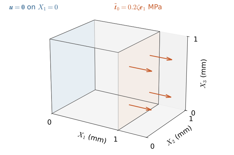
Use four subdivisions in each coordinate direction and split the cubes into tetrahedra. The displacement space is vector-valued \(P_1\). On these affine elements, the displacement gradient and the basis gradients are constant on each element, so the default quadrature integrates the internal residual and tangent terms exactly. The following blocks form one program and are intended to run sequentially in the repository’s finite-elements environment, with a single MPI process. They were checked with DOLFINx 0.11.0. The nonlinear solver interface follows the DOLFINx documentation (DOLFINx contributors, n.d.).
import numpy as np
import ufl
from mpi4py import MPI
from petsc4py import PETSc
from dolfinx import fem, mesh
from dolfinx.fem.petsc import NonlinearProblem

domain = mesh.create_unit_cube(MPI.COMM_SELF, 4, 4, 4)
V = fem.functionspace(domain, ("Lagrange", 1, (3,)))
u = fem.Function(V)
v = ufl.TestFunction(V)
w = ufl.TrialFunction(V)
fdim = domain.topology.dim - 1
left = mesh.locate_entities_boundary(domain, fdim,
    lambda x: np.isclose(x[0], 0.0))
right = mesh.locate_entities_boundary(domain, fdim,
    lambda x: np.isclose(x[0], 1.0))
fixed = fem.locate_dofs_topological(V, fdim, left)
bc = fem.dirichletbc(np.zeros(3, dtype=PETSc.ScalarType), fixed, V)
tags = mesh.meshtags(domain, fdim, np.sort(right),
    np.ones(len(right), dtype=np.int32))
ds = ufl.Measure("ds", domain=domain, subdomain_data=tags)
dx = ufl.Measure("dx", domain=domain)
The tag 1 identifies the loaded face. The facet search and degree-of-freedom location have the same roles as in Chapter 6. u stores the current displacement, v is the test function, and w is the correction direction.
9.9.2 Energy, residual, and automatic differentiation
Write the energy directly from Equation 4.68. The scalar load is the load factor \(\zeta\); it multiplies the final prescribed traction.
F = ufl.Identity(3) + ufl.grad(u)
J = ufl.det(F)
mu, lam = 1.0, 2.0
psi = mu / 2 * (ufl.tr(F.T * F) - 3) - mu * ufl.ln(J)
psi += lam / 2 * ufl.ln(J)**2
load = fem.Constant(domain, PETSc.ScalarType(0.0))
traction = ufl.as_vector((0.2, 0.0, 0.0))
Pi = psi * dx - load * ufl.dot(traction, u) * ds(1)
residual = -ufl.derivative(Pi, u, v)
tangent = ufl.derivative(residual, u, w)
The last two lines implement Equation 9.6 and Equation 9.9. In particular, residual is minus the first variation; using the first variation itself would reverse our residual convention. UFL differentiates the specified expression with respect to the coefficient u. Its automatically generated tangent can be checked against Equation 9.17 or by Equation 9.36.
9.9.3 Nonlinear solve and load increments
NonlinearProblem passes the residual and its Jacobian to PETSc’s nonlinear solver, SNES. Choose Newton iteration with backtracking, and a direct LU solve for each linear correction:
problem = NonlinearProblem(residual, u, J=tangent, bcs=[bc],
    petsc_options_prefix="c9_cube_", petsc_options={
        "snes_type": "newtonls", "snes_linesearch_type": "bt",
        "snes_atol": 1e-10, "snes_rtol": 1e-9, "snes_max_it": 20,
        "ksp_type": "preonly", "pc_type": "lu",
        "snes_error_if_not_converged": True})

for zeta in (0.25, 0.5, 0.75, 1.0):
    load.value = zeta
    problem.solve()
    if problem.solver.getConvergedReason() <= 0:
        raise RuntimeError("Nonlinear solve failed")
    u.x.scatter_forward()
    print(zeta, problem.solver.getIterationNumber())
The outer loop changes \(\zeta\). Each call to solve() keeps that load fixed and lets PETSc choose the correction factor \(\omega\) within Newton’s method. The converged solution remains in u for the next load. This short example uses prescribed increments and stops on failure. To implement the retry algorithm above, save the last converged coefficients before solve(); if a solve fails, restore them and reduce the load increment.
PETSc checks the absolute and relative residual tolerances separately, rather than adding them as in Equation 9.37. It can also report convergence when the update is small. Check the final residual norm and the reason reported by the solver (PETSc Development Team, n.d.-a). A direct LU solve is adequate for this small mesh. PETSc’s bt line search uses polynomial interpolation by default to choose trial step lengths for reducing the squared residual norm (PETSc Development Team, n.d.-b), rather than the simple halving rule above. This program does not supply a check for \(J>0\) at each trial state. The determinant checks below apply to the computed equilibria.
9.9.4 Reaction balance and deformation checks
The computed quantities should test the formulation as well as solver termination. First, the applied force on the loaded face is \(0.2\zeta A_0\bm e_1\), with \(A_0=1\) mm\(^2\). Assemble the unmodified residual before boundary rows are replaced. With this vector-valued space, fixed contains nodal block indices and each block has three components. The support reaction is minus the sum of those residual blocks:
raw_R = fem.assemble_vector(fem.form(residual)).array.copy()
reaction = -raw_R.reshape(-1, 3)[fixed].sum(axis=0)
area = fem.assemble_scalar(fem.form(1.0 * ds(1)))
applied = np.array([0.2 * float(load.value) * area, 0.0, 0.0])
print("Free residual norm:", problem.solver.getFunctionNorm())
print("Convergence reason:", problem.solver.getConvergedReason())
print("Force balance:", reaction + applied)
Second, check the element volume ratios. On affine tetrahedra with \(P_1\) displacements, \(\bF\) and \(J\) are constant on each element. A discontinuous degree-zero (DG0) function records the computed \(J\) exactly, one value per element:
Q = fem.functionspace(domain, ("DG", 0))
J_values = fem.Function(Q)
J_values.interpolate(fem.Expression(J, Q.element.interpolation_points))
mean_u1 = fem.assemble_scalar(fem.form(u[0] * ds(1))) / area
print("Minimum J:", J_values.x.array.min())
print("Mean end displacement:", mean_u1)
The diagnostic blocks above check the final converged state. Recording the same quantities after each converged load step gives the following results. Small differences in the last digits can arise from solver versions and floating-point arithmetic.
| \(\zeta\) | Newton iterations | Mean end \(u_1\) (mm) | Minimum \(J\) | Axial reaction (N) |
|---|---|---|---|---|
| 0.25 | 3 | 0.017841 | 1.004065 | \(-0.05\) |
| 0.50 | 3 | 0.036204 | 1.008179 | \(-0.10\) |
| 0.75 | 3 | 0.055103 | 1.012340 | \(-0.15\) |
| 1.00 | 3 | 0.074554 | 1.016547 | \(-0.20\) |
The reactions balance the prescribed loads, and every element has positive volume ratio at each reported state. These are useful checks, but this table does not establish mesh accuracy. To assess that accuracy, refine the mesh and compare the end displacement and other selected outputs at the same final load. The piecewise-constant \(J\) argument above also depends on the affine \(P_1\) setting and must not be reused unchanged for curved geometry or higher-degree displacement.
Exercise 9.5 (Mesh and tangent checks for the cube)
- Repeat the cube computation with two, four, and eight subdivisions per coordinate direction. At the final load, report the mean end displacement, axial reaction, and minimum \(J\). Compare successive end displacements.
- On the coarsest mesh, choose a coefficient perturbation that is zero at the clamp. Use Equation 9.36 with three decreasing values of \(\epsilon\) to check the assembled free tangent. Report the norm of the difference and its change when \(\epsilon\) is divided by ten.
9.10 Nonlinear diffusion and reaction
Consider a scalar field \(u\) on the unit square \(\Om=(0,1)^2\). The diffusion coefficient depends on the gradient of \(u\):
\[ \begin{aligned} -\divg\bigl(k(\grad u)\grad u\bigr)+c(\bx)u^3 &= f(\bx) &&\text{in }\Om,\\ u&=0 &&\text{on }\partial\Om, \end{aligned} \qquad k(\grad u)=k_0(1+|\grad u|^2). \tag{9.45}\]
Here \(k_0>0\) is constant, \(|\grad u|^2=\grad u\cdot\grad u\), \(c\in L^\infty(\Om)\) with \(c\ge0\) almost everywhere, and \(f\in L^{4/3}(\Om)\).
9.10.1 Variational problem and potential
For smooth fields, multiply Equation 9.45 by \(v\) and integrate the diffusion term by parts. Its boundary term \(-\int_{\partial\Om}v k(\grad u)\grad u\cdot\bn\,\dd s\) vanishes because \(v=0\) on \(\partial\Om\). Define the remaining terms by
\[ \begin{aligned} a(u;v)&=\int_\Om \bigl[k(\grad u)\grad u\cdot\grad v+cu^3v\bigr]\,\dx,\\ \ell(v)&=\int_\Om fv\,\dx. \end{aligned} \tag{9.46}\]
Use \(V=W^{1,4}_0(\Om)\) for both the trial and test functions, which have zero boundary values. To see why we use fourth-power integrability, note that \(|\grad u|^3\) is in \(L^{4/3}\) when \(\grad u\) is in \(L^4\): raising the former to the power \(4/3\) gives \(|\grad u|^4\). Hölder’s inequality (Equation 2.65), with exponents \(4/3\) and \(4\), gives
\[ \begin{aligned} \int_\Om |\grad u|^3|\grad v|\,\dx &\le \norm{\grad u}_{L^4}^3\norm{\grad v}_{L^4},\\ \int_\Om |cu^3v|\,\dx &\le \norm{c}_{L^\infty}\norm{u}_{L^4}^3\norm{v}_{L^4},\\ \int_\Om |fv|\,\dx &\le \norm{f}_{L^{4/3}}\norm{v}_{L^4}. \end{aligned} \]
The \(L^4\) norms are finite by the choice of \(V\). The norms of \(c\) and \(f\) are finite by assumption. The linear part of the diffusion term is also finite because \(L^4(\Om)\subset L^2(\Om)\) on the square. The cubic gradient term is the reason for using the Banach space \(W^{1,4}_0\): membership in the Hilbert space \(H^1_0\) alone does not guarantee a gradient in \(L^4\).
Find \(u\in V\) such that \(a(u;v)=\ell(v)\) for every \(v\in V\). Define \(R(u;v)=\ell(v)-a(u;v)\). The corresponding potential is
\[ \Pi(u)=\int_\Om \left[\frac{k_0}{2}|\grad u|^2+\frac{k_0}{4}|\grad u|^4 +\frac{c}{4}u^4-fu\right]\,\dx. \tag{9.47}\]
The load estimate above applies with \(u\) in place of \(v\). The other terms are finite since \(u,\grad u\in L^4\) and \(c\) is bounded. For \(u+\epsilon v\), the squared gradient has the expansion
\[ |\grad(u+\epsilon v)|^2=|\grad u|^2 +2\epsilon\grad u\cdot\grad v+\epsilon^2|\grad v|^2. \]
Thus differentiation of its square gives \(4|\grad u|^2\grad u\cdot\grad v\) at \(\epsilon=0\). Substitution in the potential and differentiation gives
\[ \begin{aligned} \delta\Pi(u;v) &=\int_\Om \bigl[k_0\grad u\cdot\grad v +k_0|\grad u|^2\grad u\cdot\grad v+cu^3v-fv\bigr]\,\dx\\ &=a(u;v)-\ell(v)=-R(u;v). \end{aligned} \tag{9.48}\]
9.10.2 Newton correction
Hold \(v\) fixed and replace \(u\) by \(u+\epsilon w\) with \(w\in V\). The load term is fixed. The derivative of \(k(\grad u+\epsilon\grad w)\) at zero is \(2k_0\grad u\cdot\grad w\). The product rule for \(k(\grad u+\epsilon\grad w)(\grad u+\epsilon\grad w)\) gives two terms, and the reaction \(c(u+\epsilon w)^3\) contributes \(3cu^2w\). The result is
\[ \begin{aligned} \delta_uR(u;v)[w]=-\int_\Om\bigl[& k(\grad u)\grad w\cdot\grad v\\ &+2k_0(\grad u\cdot\grad w)(\grad u\cdot\grad v) +3cu^2wv\bigr]\,\dx . \end{aligned} \tag{9.49}\]
For example, Hölder’s inequality with \(1/2+1/4+1/4=1\) gives
\[ \begin{aligned} \int_\Om|\grad u|^2|\grad w||\grad v|\,\dx &\le \norm{\grad u}_{L^4}^2 \norm{\grad w}_{L^4}\norm{\grad v}_{L^4},\\ \int_\Om |cu^2wv|\,\dx &\le \norm{c}_{L^\infty}\norm{u}_{L^4}^2 \norm{w}_{L^4}\norm{v}_{L^4}. \end{aligned} \]
Here \(|\grad u|^2\) and \(u^2\) are in \(L^2\) because \(u\in V\). The \(L^4\) norms of \(w,v,\grad w,\grad v\) are finite because \(w,v\in V\). The remaining term in Equation 9.49 splits into a constant coefficient term and a term bounded by the first estimate above.
Let \(\Vhzero\subset V\) consist of continuous piecewise-linear functions on triangles with zero boundary values. Find \(\Delta u_h^k\in\Vhzero\) such that
\[ \delta_uR(u_h^k;v_h)[\Delta u_h^k]=-R(u_h^k;v_h) \qquad\forall v_h\in\Vhzero . \tag{9.50}\]
Then update \(u_h^{k+1}=u_h^k+\omega\Delta u_h^k\), where \(\omega=1\) for a full Newton step. At each fixed iterate the correction equation is linear. With \(v_h=w_h\), the negative of Equation 9.49 is bounded below by \(k_0\norm{\grad w_h}_{L^2}^2\) because \(c\ge 0\). This is positive for every nonzero \(w_h\) with zero boundary values. Consequently, the negative of the free residual Jacobian is symmetric positive definite. The lower bound controls the \(H^1\) seminorm, not the \(W^{1,4}\) norm.
9.10.3 FEniCSx example
Set \(k_0=1\) and \(c(x,y)=1+x\). Choose \(u_{\mathrm{exact}}=4x(1-x)y(1-y)\), which vanishes on all four edges. Substitute it for \(u\) on the left of Equation 9.45 to obtain \(f\). In the companion notebook, UFL evaluates these spatial derivatives of the known function. The residual and its derivative with respect to the unknown are supplied explicitly, following Equation 9.46 and Equation 9.49. Here u is the current finite element function, v is a test function, and w is the trial direction for the correction:
g, gv, gw = ufl.grad(u), ufl.grad(v), ufl.grad(w)
k = k0 * (1 + ufl.dot(g, g))
ell = f * v * dx
a = (k * ufl.dot(g, gv) + c * u**3 * v) * dx
residual = ell - a
tangent = -(
    k * ufl.dot(gw, gv)
    + 2 * k0 * ufl.dot(g, gw) * ufl.dot(g, gv)
    + 3 * c * u**2 * w * v
) * dx
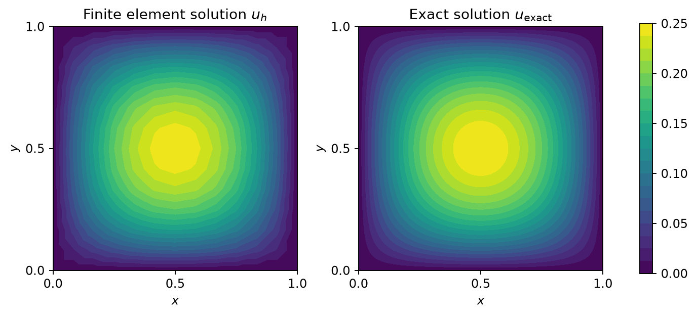
Pass residual and J=tangent to NonlinearProblem together with the zero Dirichlet condition, as in Section 9.9. The notebook starts from zero and calls solve() once at the full load, using PETSc Newton iteration with backtracking. On the mesh with \(288\) triangles, the solver took seven Newton iterations and the computed \(L^2\) error was \(2.1808\times10^{-3}\). Figure 9.4 compares the two solutions on the same color scale.
9.11 Chapter summary
- Hyperelastic equilibrium is \(R(\bu;\bv)=\ell_{\mathrm{hyp}}(\bv) -a_{\mathrm{hyp}}(\bu;\bv)=0\) for every admissible test function. The potential satisfies \(\delta\Pi=-R\) and its second variation is the negative of the residual derivative.
- Newton’s method linearizes the residual at the current displacement and solves \(\delta_uR[\Delta\bu]=-R\). Corrections have zero prescribed displacement when the current iterate satisfies the fixed boundary data.
- Consistent differentiation of the stress law produces the material tangent. Linearizing before discretization and differentiating the assembled residual give the same matrix when quadrature and boundary treatment agree.
- The assembled Jacobian is \(\bK_T=\partial\bR/\partial\bU\). Solve \((K_T)_{ff}\Delta\bU_f=-\bR_f\), retain the prescribed coefficients, and recover support reactions as \(-\bR_p\).
- Load stepping changes the load between equilibrium solves and uses a previous equilibrium as the next initial guess. Backtracking keeps the load fixed and reduces a correction when the full update is unsuitable.
- Residual convergence, tangent verification, positive deformation determinants, force balance, and mesh accuracy are distinct checks. UFL supplies derivatives of the stated forms; those checks remain necessary.
- For nonlinear diffusion, the cubic gradient term calls for \(W^{1,4}_0(\Om)\) in the continuous problem. The residual and its tangent can be written directly in UFL and passed to the same nonlinear solver.