3 Partial Differential Equations and Variational Formulations
A finite element approximation begins with a variational problem. The variational problem is obtained from a boundary-value problem by introducing test functions, integrating over the domain, and transferring derivatives by integration by parts. This process also determines how the boundary conditions enter the formulation and which function spaces contain the unknown and the test functions.
Chapter 2 introduced the mathematical objects needed for this construction. This chapter uses them to develop the formulation procedure for a scalar diffusion problem. The same procedure will be applied to heat conduction and solid mechanics in Chapter 4.
3.1 Boundary-value problems and variational statements
A boundary-value problem specifies a domain, an unknown field, a differential equation in the domain, and conditions on the boundary. Its data include the coefficients and source terms in the equation and the values or fluxes prescribed on the boundary. All of these items are part of the mathematical problem.
3.1.1 Strong form and solution terminology
The differential equation together with its boundary conditions is called the strong form of the boundary-value problem. In this book, a strong solution, or classical solution, has enough pointwise differentiability to satisfy that equation and its boundary conditions in the classical sense. The required regularity depends on the differential operator and the coefficients.
Many finite element functions are continuous across cell boundaries but do not have the classical second derivatives required by a second-order differential equation. The variational formulation reduces the required derivative order and leads to the definition of a weak solution.
3.1.2 Abstract strong and variational problems
Let \(\mathcal{L}\) be a differential operator that may depend linearly or nonlinearly on \(u\). Two examples are
\[ \mathcal{L}(u)(\bx)=-\Delta u(\bx) \quad\text{(linear)}, \qquad \mathcal{L}(u)(\bx)=-\Delta u(\bx)+\sin\bigl(u(\bx)\bigr) \quad\text{(nonlinear)}. \]
In the equations above, \(\Delta\) is the Laplacian and is defined by \(\Delta u(\bx)=\nabla\cdot(\nabla u(\bx))\).
Suppose \(\partial\Om\) is divided into two portions, \(\Gam_D\) and \(\Gam_N\), and let \(\bm q(u)\) denote the flux associated with the differential equation. The abstract strong problem is
\[ \left. \begin{aligned} \mathcal{L}(u)(\bx)&=f(\bx) &&\forall\bx\in\Om,\\ u(\bx)&=g(\bx) &&\forall\bx\in\Gam_D,\\ \bm q(u)(\bx)\cdot\bn(\bx)&=h(\bx) &&\forall\bx\in\Gam_N. \end{aligned} \right\} \qquad\text{Strong form} \tag{3.1}\]
The second equation prescribes the value of \(u\) on \(\Gam_D\). The third prescribes the component of the flux normal to the boundary on \(\Gam_N\), where \(\bn(\bx)\) is the outward unit normal at \(\bx\in\partial\Om\).
The corresponding abstract variational problem uses a trial space \(\mathcal U_g\) and a test space \(\mathcal V_0\):
\[ \left. \begin{aligned} &\text{Find }u\in\mathcal U_g\text{ such that}\\ &a(u;v)=\ell(v) \qquad\forall v\in\mathcal V_0. \end{aligned} \right\} \qquad\text{Variational form} \tag{3.2}\]
The trial space \(\mathcal U_g\) contains functions satisfying \(u=g\) on \(\Gam_D\), and the test space \(\mathcal V_0\) contains functions satisfying \(v=0\) on \(\Gam_D\). We next explain how the variational form follows from the strong form.
For a candidate field \(u\), define the residual at \(\bx\in\Om\) by
\[ R(u)(\bx)=\mathcal{L}(u)(\bx)-f(\bx). \]
A strong solution satisfies
\[ R(u)(\bx)=0 \qquad\forall\bx\in\Om. \]
Multiplying this equation by a weighting function \(v(\bx)\) and integrating over \(\Om\) gives
\[ \int_{\Om}v(\bx)R(u)(\bx)\,\dx=0. \tag{3.3}\]
This is a weighted residual statement. The weighting function becomes the test function in the variational problem. Requiring Equation 3.3 for one function \(v\) would give only one scalar condition. It must hold for every function in a specified test space.
For a second-order equation, integration by parts transfers one derivative from the candidate field to the test function and introduces boundary terms. After the prescribed normal flux \(h\) is substituted on \(\Gam_N\), the resulting equation has the form stated in Equation 3.2. The form \(a\) contains the terms involving the unknown, while \(\ell\) contains the prescribed source \(f\) and flux \(h\).
If \(\mathcal L\) and the flux \(\bm q\) depend linearly on \(u\), then \(a\) is bilinear and is written \(a(u,v)\). If \(\mathcal L\) or \(\bm q\) depends nonlinearly on \(u\), then \(a\) is generally nonlinear in the trial argument but remains linear in the test argument. It is written \(a(u;v)\) and is semilinear in the sense of Definition 2.24. The semicolon identifies the argument in which nonlinear dependence is allowed.
Remark 3.1 (Weak identity and variational problem). An integral equation alone does not define a variational problem. The spaces containing the unknown and the test functions determine the boundary values, regularity, and admissible variations. They are part of the formulation.
Figure 3.1 summarizes the steps. Each arrow represents a mathematical operation or choice that must be stated in the formulation.

3.2 Canonical scalar diffusion problem
We now carry out the complete procedure for a scalar diffusion equation. The problem is used here as a mathematical prototype. Chapter 4 develops its heat conduction interpretation from the corresponding physical balance law.
3.2.1 Strong boundary-value problem
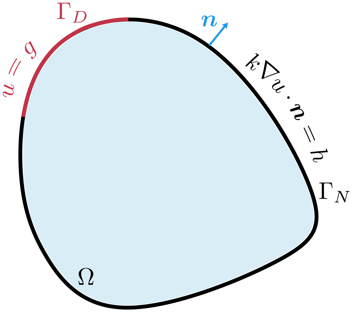
Let \(\Om\subset\R^d\) be a bounded Lipschitz domain. Let \(\Gam_D\) and \(\Gam_N\) be disjoint portions that are open relative to \(\partial\Om\) and whose closures cover the boundary:
\[ \partial\Om=\overline{\Gam_D}\cup\overline{\Gam_N}, \qquad \Gam_D\cap\Gam_N=\varnothing. \tag{3.4}\]
Assume that the interface \(\overline{\Gam_D}\cap\overline{\Gam_N}\) has boundary measure zero and that \(\Gam_D\) has positive boundary measure. The partition and the outward unit normal are shown schematically in Figure 3.2.
Consider
\[ \bigl[-\divg(k\grad u)\bigr](\bx)=f(\bx) \qquad\forall\bx\in\Om, \tag{3.5}\]
with boundary conditions
\[ u(\bx)=g(\bx) \quad\forall\bx\in\Gam_D, \qquad k(\bx)\grad u(\bx)\cdot\bn(\bx)=h(\bx) \quad\forall\bx\in\Gam_N. \tag{3.6}\]
The condition on \(\Gam_D\) prescribes the value of \(u\). The condition on \(\Gam_N\) prescribes the component of \(k\grad u\) normal to the boundary, which we call the normal flux for this prototype problem.
In the integral equations below, the explicit dependence on \(\bx\) is suppressed. Thus, for example, \(k\grad u\) denotes the vector field \(\bx\mapsto k(\bx)\grad u(\bx)\).
To interpret this problem classically, suppose that \(\partial\Om\) is of class \(C^1\), so that the outward unit normal \(\bn\) is defined pointwise on \(\partial\Om\). Let
\[ k\in C^1(\Om)\cap C(\overline{\Om}), \qquad k(\bx)\geq k_0>0, \qquad f\in C(\Om), \]
with boundary data
\[ g\in C(\overline{\Gam_D}), \qquad h\in C(\overline{\Gam_N}), \]
and suppose that a solution \(u\in C^2(\Om)\cap C^1(\overline{\Om})\) exists. Then \(\divg(k\grad u)\) is defined pointwise in \(\Om\), while \(u\) and \(k\grad u\cdot\bn\) are defined pointwise on the corresponding portions of the boundary. Hence Equation 3.5 and Equation 3.6 can be imposed in the classical sense.
These regularity assumptions need not hold in applications. A material coefficient may be discontinuous, and source and flux data may have limited regularity. We therefore replace the classical assumptions by
\[ k\in L^\infty(\Om), \qquad 0<k_0\leq k(\bx)\leq k_1<\infty \quad\text{for almost every }\bx\in\Om, \tag{3.7}\]
and let \(f\in L^2(\Om)\) and \(h\in L^2(\Gam_N)\). We also assume that there is at least one function \(u_g\in H^1(\Om)\) with boundary value \(g\) on \(\Gam_D\). This last assumption ensures that the trial space introduced below is nonempty.
Under these weaker assumptions, a solution need not belong to \(C^2(\Om)\), and Equation 3.5 need not be meaningful at every \(\bx\in\Om\). We therefore seek a weak solution defined by an integral equation.
3.2.2 Weighted residual and integration by parts
Begin with a smooth weighting function \(v\) satisfying
\[ v(\bx)=0 \qquad\forall\bx\in\Gam_D. \]
Multiplication of Equation 3.5 by \(v\) and integration over \(\Om\) gives
\[ -\int_{\Om}v\,\divg(k\grad u)\,\dx -\int_{\Om}fv\,\dx=0. \tag{3.8}\]
Equivalently,
\[ -\int_{\Om}v\,\divg(k\grad u)\,\dx =\int_{\Om}fv\,\dx. \]
Apply Green’s formula in Equation 2.39 with the vector field \(k\grad u\). The complete identity is
\[ \int_{\Om}k\grad u\cdot\grad v\,\dx -\int_{\partial\Om}v\,k\grad u\cdot\bn\,\ds =\int_{\Om}fv\,\dx. \tag{3.9}\]
Using the boundary partition in Equation 3.4, the boundary contribution is
\[ -\int_{\partial\Om}v\,k\grad u\cdot\bn\,\ds = -\int_{\Gam_D}v\,k\grad u\cdot\bn\,\ds -\int_{\Gam_N}v\,k\grad u\cdot\bn\,\ds. \]
The first integral is zero because \(v=0\) on \(\Gam_D\). On \(\Gam_N\), substitute \(k\grad u\cdot\bn=h\). Equation Equation 3.9 then becomes
\[ \int_{\Om}k\grad u\cdot\grad v\,\dx =\int_{\Om}fv\,\dx+\int_{\Gam_N}hv\,\ds. \tag{3.10}\]
The highest derivative of \(u\) in this identity is its first derivative. This reduction from second to first derivatives determines the appropriate function space for the formulation.
3.2.3 Trial and test spaces
We now choose the space containing the solution, called the trial space, and the space containing the weighting functions, called the test space. They must be chosen so that every term in Equation 3.10 is well defined; in particular, each integral must be finite for the assumed \(k\), \(f\), and \(h\).
By the \(p=q=2\) case of the Hölder inequality in Theorem 2.8, the source term satisfies
\[ \left|\int_{\Om}fv\,\dx\right| \leq \norm{f}_{L^2(\Om)}\norm{v}_{L^2(\Om)}. \tag{3.11}\]
Thus the source term is finite when \(v\in L^2(\Om)\). For the left-hand side, the upper bound on \(k\) in Equation 3.7 and another application of Hölder give
\[ \left|\int_{\Om}k\grad u\cdot\grad v\,\dx\right| \leq \norm{k}_{L^\infty(\Om)} \norm{\grad u}_{L^2(\Om;\R^d)} \norm{\grad v}_{L^2(\Om;\R^d)}. \tag{3.12}\]
Consequently, \(u\) and \(v\) should have first-order weak derivatives in \(L^2(\Om;\R^d)\). Combining this requirement with \(u,v\in L^2(\Om)\) gives \(u,v\in H^1(\Om)\). The Neumann term is also finite for such test functions. Indeed, Hölder on \(\Gam_N\) and the trace inequality Theorem 2.10 give
\[ \left|\int_{\Gam_N}hv\,\ds\right| \leq \norm{h}_{L^2(\Gam_N)}\norm{v}_{L^2(\Gam_N)} \leq C_{\mathrm{tr}}\norm{h}_{L^2(\Gam_N)}\norm{v}_{H^1(\Om)}. \tag{3.13}\]
The derivation of Equation 3.10 additionally requires the test function to vanish on \(\Gam_D\). We therefore choose
\[ \Vzero =\{v\in H^1(\Om):v=0\text{ on }\Gam_D\} =H^1_{0,\Gam_D}(\Om) \tag{3.14}\]
as the test space. The solution must instead satisfy the prescribed value \(u=g\) on \(\Gam_D\), which gives the trial space
\[ \Ug =\{w\in H^1(\Om):w=g\text{ on }\Gam_D\}. \tag{3.15}\]
The boundary-value notation uses the convention introduced in Remark 2.10.
The space \(\Vzero\) is a vector space. Because the boundary-value mapping is continuous, the functions with zero boundary value on \(\Gam_D\) form a closed subspace of \(H^1(\Om)\). Thus \(\Vzero\) is a Hilbert space with the \(H^1\) inner product and norm. When \(g\ne0\), however, \(\Ug\) does not contain the zero function and is not a vector space; more precisely, it is an affine space of the form \(u_g+\Vzero\).
With these spaces specified, the weak formulation is to find \(u\in\Ug\) such that
\[ \int_{\Om}k\grad u\cdot\grad v\,\dx =\int_{\Om}fv\,\dx+\int_{\Gam_N}hv\,\ds \qquad\forall v\in\Vzero. \tag{3.16}\]
3.2.4 Variational problem
In Equation 3.16, the left-hand side depends on both \(u\) and \(v\), whereas the right-hand side depends only on \(v\). This structure leads naturally to a bilinear form \(a\) and a linear functional \(\ell\), defined by
\[ a(w,v)=\int_{\Om}k\grad w\cdot\grad v\,\dx, \qquad \ell(v)=\int_{\Om}fv\,\dx+\int_{\Gam_N}hv\,\ds. \tag{3.17}\]
Definition 3.1 (Variational diffusion problem) Find \(u\in\Ug\) such that
\[ a(u,v)=\ell(v) \qquad\forall v\in\Vzero. \tag{3.18}\]
A function \(u\in\Ug\) that satisfies this problem is a weak solution of the boundary-value problem. No mesh or finite-dimensional approximation has been introduced. Both \(\Ug\) and \(\Vzero\) remain infinite dimensional.
The notation also displays the general structure of a variational problem. If \(\mathcal{U}\) is a trial space, \(\mathcal{V}\) is a test space, \(a:\mathcal{U}\times\mathcal{V}\to\R\), and \(\ell:\mathcal{V}\to\R\), the problem is to find \(u\in\mathcal{U}\) such that \(a(u,v)=\ell(v)\) for every \(v\in\mathcal{V}\). The spaces and the two forms must be specified for each problem.
Example 3.1 (A one-dimensional variational problem) Let \(\Om=(0,1)\) and consider
\[ -u''(x)=1 \qquad 0<x<1, \]
with boundary conditions
\[ u(0)=0, \qquad u'(1)=0. \]
The trial and test spaces are the same in this homogeneous problem:
\[ \Ug=\Vzero=\{v\in H^1(0,1):v(0)=0\}. \]
Multiplying the differential equation by \(v\in\Vzero\) and integrating by parts gives
\[ \int_0^1u'v'\,\dd x-[vu']_0^1=\int_0^1v\,\dd x. \]
The endpoint term is zero: \(v(0)=0\) at the Dirichlet endpoint and \(u'(1)=0\) at the Neumann endpoint. The variational problem is therefore
\[ \text{find }u\in\Ug\text{ such that}\qquad \int_0^1u'v'\,\dd x=\int_0^1v\,\dd x \quad\forall v\in\Vzero. \]
The classical solution is \(u(x)=x-\tfrac12x^2\). Since \(u'(x)=1-x\),
\[ \int_0^1u'v'\,\dd x =\int_0^1(1-x)v'\,\dd x =[(1-x)v]_0^1+\int_0^1v\,\dd x =\int_0^1v\,\dd x, \]
where \(v(0)=0\). Thus the classical solution also satisfies the variational problem.
Exercise 3.1 (Diffusion with a fully Dirichlet boundary) Set \(\Gam_D=\partial\Om\) and prescribe \(u=0\) on \(\partial\Om\).
- State the trial and test spaces.
- Starting from Equation 3.9, identify the boundary integral that vanishes and state why it is zero.
- State the resulting bilinear form, linear functional, and variational problem.
3.2.5 Essential, natural, and Robin boundary conditions
The condition \(u=g\) on \(\Gam_D\) is called an essential boundary condition because it is imposed through membership in \(\Ug\). The corresponding test function has the homogeneous value \(v=0\) on \(\Gam_D\).
The condition \(k\grad u\cdot\bn=h\) on \(\Gam_N\) is called a natural boundary condition because it enters through the boundary integral produced by integration by parts. It contributes to \(\ell(v)\) but does not restrict the test functions on \(\Gam_N\). The terms essential and natural describe how the conditions enter the variational problem; they do not rank their physical importance.
A Robin condition combines the unknown and its normal flux. If
\[ k(\bx)\grad u(\bx)\cdot\bn(\bx) +\beta(\bx)u(\bx)=r(\bx) \qquad\forall\bx\in\Gam_N, \]
then \(k\grad u\cdot\bn=r-\beta u\). Substitution into Equation 3.9 gives
\[ \int_{\Om}k\grad u\cdot\grad v\,\dx +\int_{\Gam_N}\beta uv\,\ds =\int_{\Om}fv\,\dx+\int_{\Gam_N}rv\,\ds. \tag{3.19}\]
Thus the term containing the unknown \(u\) belongs to the bilinear form, while the prescribed datum \(r\) belongs to the linear functional.
Exercise 3.2 (A Robin boundary condition) Assume \(\beta\in L^\infty(\Gam_N)\) with \(\beta\geq0\) almost everywhere and \(r\in L^2(\Gam_N)\). For the Robin condition above:
- derive Equation 3.19 from Equation 3.9;
- state the trial and test spaces;
- state the complete bilinear form and linear functional.
Remark 3.2 (When only flux is prescribed). If \(\Gam_D\) is empty, the boundary condition prescribes only the flux. This is called a pure Neumann problem. Adding a constant \(c\) to \(u\) does not change \(\grad u\), so \(u\) and \(u+c\) satisfy the same differential equation and flux condition. The solution is therefore not unique unless its constant value is fixed in some other way.
The prescribed data must also satisfy a compatibility condition. Set \(\Gam_N=\partial\Om\) and \(v=1\) in Equation 3.16. Because \(\grad v=0\), the equation gives
\[ \int_{\Om}f\,\dx+\int_{\partial\Om}h\,\ds=0. \]
When this condition holds, a requirement such as \(\int_{\Om}u\,\dx=0\) selects one solution. In the problem considered above, \(\Gam_D\) has positive boundary measure and the prescribed value on \(\Gam_D\) fixes the additive constant.
3.3 Weak solutions and the differential problem
The derivation above proves one implication directly: any sufficiently smooth solution of the strong boundary-value problem satisfies the variational problem. We now establish the reverse implication under classical regularity.
Let \(u\in\Ug\) satisfy the variational problem Equation 3.16. Assume that \(u\), \(k\), and the data have enough regularity for \(\divg(k\grad u)\) to be continuous in \(\Om\) and for integration by parts to hold classically. To recover the differential equation at points inside \(\Om\), choose a test function \(v\in C_0^\infty(\Om)\) as defined in Definition 2.16. Because \(v\) is zero near \(\partial\Om\), integration by parts produces no boundary contribution, and Equation 3.16 gives
\[ \int_{\Om} \bigl[-\divg(k\grad u)-f\bigr]v\,\dx=0 \qquad\forall v\in C_0^\infty(\Om). \]
By the fundamental lemma Theorem 2.2, the expression \(-\divg(k\grad u)-f\) is zero almost everywhere. This expression is continuous under the regularity assumed above, so it is zero at every point in \(\Om\). Hence
\[ \bigl[-\divg(k\grad u)\bigr](\bx)=f(\bx) \qquad\forall\bx\in\Om. \]
This is the differential equation Equation 3.5 in pointwise form. Substituting it into the integration-by-parts identity for a general \(v\in\Vzero\) gives
\[ \int_{\Gam_N}v \bigl(k\grad u\cdot\bn-h\bigr)\,\ds=0. \]
No value is prescribed for \(v\) on \(\Gam_N\), so the boundary value of \(v\) can be varied there. Under classical boundary regularity, the identity therefore implies
\[ k(\bx)\grad u(\bx)\cdot\bn(\bx)=h(\bx) \qquad\forall\bx\in\Gam_N. \]
The condition \(u=g\) on \(\Gam_D\) already follows from \(u\in\Ug\). Thus the weak solution satisfies the differential equation at every point in \(\Om\) and both boundary conditions when the required classical regularity is available. Without this regularity, Equation 3.18 remains meaningful and defines the weak solution (Süli 2012; Larson and Bengzon 2010).
Example 3.2 (A weak solution with a discontinuous coefficient) Let \(\Om=(0,1)\), prescribe \(u(0)=0\) and \(u(1)=1\), and set
\[ k(x)= \begin{cases} 1, & 0<x<\tfrac12,\\ 2, & \tfrac12<x<1. \end{cases} \]
For \(f=0\), define
\[ u(x)= \begin{cases} \dfrac43x, & 0\leq x\leq\tfrac12,\\[0.4em] \dfrac23+\dfrac23\left(x-\tfrac12\right), & \tfrac12\leq x\leq1. \end{cases} \]
The function \(u\) is continuous and belongs to \(H^1(0,1)\), but its derivative jumps at \(x=1/2\). The test space is
\[ H_0^1(0,1) =\{v\in H^1(0,1):v(0)=v(1)=0\}. \]
Here the subscript \(0\) indicates that \(v=0\) on the entire boundary \(\partial\Om=\{0,1\}\). On both subintervals, \(ku'=4/3\). Therefore, for every \(v\in H_0^1(0,1)\),
\[ \int_0^1ku'v'\,\dd x =\frac43\int_0^1v'\,\dd x =\frac43[v(1)-v(0)]=0. \]
The right-hand side of Equation 3.16 is zero because \(f=0\) and \(\Gam_N\) is empty. Thus \(u\) satisfies Equation 3.16 with \(\Gam_D=\partial\Om\). This example shows why continuity of the flux \(ku'\), rather than continuity of \(u'\), is the relevant interface condition for this diffusion problem.
3.4 Well-posedness and stability
We now ask whether the variational problem has a unique solution and whether that solution depends continuously on \(f\) and \(h\). For this discussion, assume \(g=0\). The trial and test spaces are then the same Hilbert space, \(\Ug=\Vzero\), equipped with the \(H^1(\Om)\) norm, and the problem is
\[ \text{find }u\in\Vzero\text{ such that}\qquad a(u,v)=\ell(v) \quad\forall v\in\Vzero. \tag{3.20}\]
The Lax–Milgram theorem Theorem 2.4 gives existence, uniqueness, and a stability estimate for a problem of this form once we verify that \(a\) is continuous and coercive and that \(\ell\) is a continuous linear functional. We verify these three requirements next.
For \(w,v\in\Vzero\), the bilinear form is
\[ a(w,v)=\int_{\Om}k\grad w\cdot\grad v\,\dx. \]
The coefficient upper bound in Equation 3.7 and the Cauchy–Schwarz inequality Theorem 2.6 give
\[ \begin{aligned} |a(w,v)| &=\left|\int_{\Om}k\grad w\cdot\grad v\,\dx\right|\\ &\leq k_1 \norm{\grad w}_{L^2(\Om;\R^d)} \norm{\grad v}_{L^2(\Om;\R^d)}\\ &\leq k_1 \norm{w}_{H^1(\Om)} \norm{v}_{H^1(\Om)}. \end{aligned} \tag{3.21}\]
Thus the bilinear form \(a\) is continuous on \(\Vzero\times\Vzero\) according to Definition 2.26, with continuity constant \(M=k_1\).
For \(v\in\Vzero\), the coefficient lower bound and the Poincare inequality Theorem 2.11 give
\[ \begin{aligned} a(v,v) &=\int_{\Om}k|\grad v|^2\,\dx\\ &\geq k_0\norm{\grad v}_{L^2(\Om;\R^d)}^2\\ &\geq \frac{k_0}{1+C_P^2} \norm{v}_{H^1(\Om)}^2 \qquad\forall v\in\Vzero. \end{aligned} \tag{3.22}\]
Therefore the bilinear form \(a\) is coercive on \(\Vzero\) according to Definition 2.27, with coercivity constant \(\alpha=k_0/(1+C_P^2)\). The positive-measure assumption on \(\Gam_D\) is needed here because it is one of the hypotheses of the Poincare inequality.
For the linear functional \(\ell\), the Cauchy–Schwarz inequality and the trace inequality Theorem 2.10 give
\[ \begin{aligned} |\ell(v)| &\leq \norm{f}_{L^2(\Om)}\norm{v}_{L^2(\Om)} +\norm{h}_{L^2(\Gam_N)}\norm{v}_{L^2(\Gam_N)}\\ &\leq \left( \norm{f}_{L^2(\Om)} +C_{\mathrm{tr}}\norm{h}_{L^2(\Gam_N)} \right) \norm{v}_{H^1(\Om)}. \end{aligned} \tag{3.23}\]
The characterization in Theorem 2.3 shows that \(\ell\) is continuous on \(\Vzero\) and hence belongs to the dual space \(\Vzero^*\).
All hypotheses of the Lax–Milgram theorem Theorem 2.4 are now satisfied. Therefore Equation 3.20 has a unique weak solution \(u\in\Vzero\). The stability estimate supplied by the theorem is
\[ \norm{u}_{H^1(\Om)} \leq \frac{1}{\alpha} \left( \norm{f}_{L^2(\Om)} +C_{\mathrm{tr}}\norm{h}_{L^2(\Gam_N)} \right). \tag{3.24}\]
The case \(g\ne0\) requires an additional step because \(\Ug\) is an affine set, not the Hilbert space used in Theorem 2.4. We defer that construction to the treatment of nonhomogeneous finite element boundary data in Chapter 5.
Exercise 3.3 (Estimates for the diffusion problem)
- Prove Equation 3.21 using the coefficient upper bound and the Cauchy–Schwarz inequality Theorem 2.6.
- Prove Equation 3.22 using the coefficient lower bound and the Poincare inequality Theorem 2.11.
- Prove Equation 3.23 using the Cauchy–Schwarz inequality and the trace inequality Theorem 2.10.
- Use the three estimates to derive Equation 3.24.
- Explain which step fails for the pure Neumann problem when constants remain in the test space.
3.5 Energy minimization and first variation
The variational diffusion problem was derived directly from the strong problem by multiplying the differential equation by a test function and integrating by parts. No energy functional was required.
We now show that the particular variational problem in Definition 3.1, where \(a(u,v)\) and \(\ell(v)\) are defined in Equation 3.17, can be obtained from an energy functional. Whenever this is possible, we say that the problem has an energy structure. We show that:
- the variational equation is the stationarity condition of an energy functional; and
- because the diffusion form is symmetric and coercive, the weak solution is the unique minimizer of that energy.
Return to the general trial space \(\Ug\), which may include nonzero essential boundary data. Define
\[ \Pi(z)=\frac12a(z,z)-\ell(z), \qquad z\in\Ug. \tag{3.25}\]
The quadratic term is the field contribution, and \(\ell(z)\) is the contribution from the prescribed data. We call their difference the total energy functional for this prototype problem. Its physical interpretation depends on the governing model; Chapter 4 develops that interpretation for heat conduction and solid mechanics.
Let \(u\in\Ug\). A permissible variation must preserve the prescribed boundary value. Therefore, if \(v\in\Vzero\), then \(u+\epsilon v\in\Ug\) for every scalar \(\epsilon\). Indeed, \(v=0\) on \(\Gam_D\), so \(u+\epsilon v=g\) on \(\Gam_D\). Symmetry and bilinearity give
\[ \Pi(u+\epsilon v)-\Pi(u) =\epsilon\bigl(a(u,v)-\ell(v)\bigr) +\frac{\epsilon^2}{2}a(v,v). \tag{3.26}\]
Using the definition of first variation in Definition 2.25, divide the preceding equation by \(\epsilon\) and take the limit as \(\epsilon\to0\). The first variation of the energy functional is
\[ \delta\Pi(u;v) =a(u,v)-\ell(v). \tag{3.27}\]
A stationary point is one at which the first variation is zero in every permissible direction. This condition alone does not distinguish a minimum from a maximum. The stationarity condition for \(\Pi\) is
\[ \delta\Pi(u;v)=0 \qquad\forall v\in\Vzero. \tag{3.28}\]
The above is exactly the variational equation \(a(u,v)=\ell(v)\) for every \(v\in\Vzero\). Thus the variational problem can be obtained by taking the first variation of \(\Pi\) and setting it to zero.
Now suppose that \(u\) satisfies \(\delta\Pi(u;v)=0\) for every \(v\in\Vzero\). For any \(v\in\Vzero\), set \(\epsilon=1\) in Equation 3.26. Then
\[ \Pi(u+v)-\Pi(u) =\bigl(a(u,v)-\ell(v)\bigr)+\frac{1}{2}a(v,v) =\frac{1}{2}a(v,v). \tag{3.29}\]
Coercivity implies that \(a(v,v)>0\) for every nonzero \(v\in\Vzero\), while \(a(0,0)=0\). Therefore, Equation 3.29 is positive for every nonzero permissible variation. It follows that \(u\) is the unique minimizer of \(\Pi\) over \(\Ug\).
Remark 3.3 (Variational problem is more general). A variational form can be derived from a strong differential equation through a weighted residual statement and integration by parts without introducing an energy. An energy formulation requires a functional \(\Pi\) whose first variation reproduces the variational equation:
\[ \delta\Pi(u;v)=a(u;v)-\ell(v). \tag{3.30}\]
Such a functional need not exist. For example, let \(a\) be a nonsymmetric bilinear form and define \(J(u):=(1/2)a(u,u)\). Its first variation is
\[ \delta J(u;v) =\frac12\bigl(a(u,v)+a(v,u)\bigr), \]
which does not reproduce \(a(u,v)\) unless \(a(u,v) = a(v,u)\), i.e., unless \(a\) is symmetric. Similarly, a nonlinear semilinear form \(a(u;v)\) admits an energy formulation only when it is the first variation of some scalar functional. Therefore the variational formulation is more general than energy minimization. When a suitable energy exists and has the required convexity, the variational problem and energy minimization give the same solution (Jog 1978).
Remark 3.4 (Energy functional for a symmetric bilinear form). Suppose that \(a\) is a symmetric bilinear form and \(\ell\) is a linear functional. Then
\[ \Pi(z)=\frac12a(z,z)-\ell(z) \]
has first variation \(\delta\Pi(u;v)=a(u,v)-\ell(v)\). Its stationarity condition is therefore equivalent to the variational equation \(a(u,v)=\ell(v)\) for every \(v\in\Vzero\). Symmetry provides this energy structure; positive definiteness or coercivity is additionally needed to conclude that the stationary point is a unique minimizer.
Exercise 3.4 (First variation and the minimum property)
- Starting from Equation 3.25, derive Equation 3.26.
- Divide the expansion by \(\epsilon\) and compute \(\delta\Pi(u;v)\) from the definition of the first variation.
- Show that a minimizer of \(\Pi\) satisfies Equation 3.28 and hence the variational problem.
- Assume that \(u\) satisfies the variational problem and derive Equation 3.29.
- Use coercivity to prove that \(u\) is the unique minimizer of \(\Pi\) over \(\Ug\).
3.6 A nonlinear problem and its semilinear form
The scalar diffusion problem above is linear in \(u\) and leads to the bilinear form \(a(u,v)\). For comparison, consider the nonlinear problem
\[ \left. \begin{aligned} -\Delta u(\bx)+\sin\bigl(u(\bx)\bigr)&=f(\bx) &&\forall\bx\in\Om,\\ u(\bx)&=0 &&\forall\bx\in\partial\Om. \end{aligned} \right\} \qquad\text{Strong form} \tag{3.31}\]
Assume that \(\Om\) is bounded and \(f\in L^2(\Om)\). Multiplication by \(v\in H_0^1(\Om)\) and integration by parts give
\[ \int_{\Om}\grad u\cdot\grad v\,\dx +\int_{\Om}(\sin u)v\,\dx =\int_{\Om}fv\,\dx. \]
Define
\[ a(u;v) =\int_{\Om}\grad u\cdot\grad v\,\dx +\int_{\Om}(\sin u)v\,\dx, \qquad \ell(v)=\int_{\Om}fv\,\dx. \tag{3.32}\]
The corresponding variational problem is
\[ \left. \begin{aligned} &\text{Find }u\in H_0^1(\Om)\text{ such that}\\ &a(u;v)=\ell(v) \qquad\forall v\in H_0^1(\Om). \end{aligned} \right\} \qquad\text{Variational form} \tag{3.33}\]
The form \(a(u;v)\) is nonlinear in \(u\) because of \(\sin u\), but it is linear in \(v\). It is therefore semilinear. The reaction term is well defined because \(|\sin u|\leq1\), so \(\sin u\in L^2(\Om)\) on a bounded domain.
3.7 From the continuous problem to FEM
The variational problem is still infinite dimensional. A conforming finite element method for the homogeneous problem Equation 3.20 chooses a finite-dimensional space \(\Vh\subset\Vzero\). The discrete problem is
\[ \text{find }\uh\in\Vh\text{ such that}\qquad a(\uh,\vh)=\ell(\vh) \quad\forall\vh\in\Vh. \tag{3.34}\]
Chapter 4 supplies the continuum models to which this formulation will be applied. Chapter 5 constructs the finite-dimensional spaces, explains how homogeneous and nonhomogeneous boundary data are represented, and derives the corresponding algebraic systems.
3.8 Chapter summary
- A boundary-value problem specifies the differential equation, coefficients, sources, and boundary conditions on a stated domain.
- Integration by parts converts the weighted residual statement to a weak identity. The trial and test spaces complete the variational problem and determine how essential and natural boundary data enter it.
- A linear differential operator commonly produces a bilinear form. A nonlinear operator generally produces a semilinear form that is nonlinear in the trial argument and linear in the test argument.
- For homogeneous essential data, continuity and coercivity of the bilinear form and continuity of the load functional allow the Lax–Milgram theorem to establish existence, uniqueness, and stability.
- For symmetric diffusion, the variational equation is equivalent to energy minimization over the admissible affine space. An energy functional is additional structure and need not exist for a general variational problem.