6 Finite Element Approximation in Multiple Dimensions
Chapter 5 developed the finite element method on an interval. The essential ideas were local even though the final algebraic problem was global: divide the domain into elements, construct polynomial basis functions on those elements, join neighboring pieces through shared degrees of freedom, evaluate the variational problem element by element, and assemble the local contributions into one sparse system.
The same structure carries over to two and three dimensions. What changes is the geometry. An interval element has two endpoints and one spatial coordinate. A triangle or tetrahedron has several facets and requires more than one coordinate; a quadrilateral or hexahedron introduces tensor-product basis functions and generally nonconstant geometry mappings. Gradients must be transformed between physical and reference coordinates, and natural boundary terms are integrated over element facets rather than over endpoints.
This chapter develops those changes without restarting the finite element method from the beginning. We first construct a linear triangular element directly on a physical triangle, then build the corresponding global space and discrete scalar-diffusion problem. Only after that construction is clear do we introduce reference cells, Jacobians, multidimensional quadrature, and isoparametric mappings. The final sections extend the scalar construction to vector-valued elasticity and connect the mathematical objects to their FEniCSx counterparts. The presentation follows the physical-element and local-to-global constructions commonly used in finite element texts and lecture notes (Jog 1978; Larson and Bengzon 2010; Arnold 2011).
6.1 From intervals to multidimensional meshes
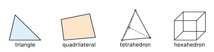
Let \(\Om\subset\R^d\), with \(d=2\) or \(3\), be the computational domain. In one dimension, the mesh consisted of intervals. In multiple dimensions, the domain is partitioned into cells. Typical two-dimensional cells are triangles and quadrilaterals; typical three-dimensional cells are tetrahedra and hexahedra. For the straight-sided cells developed first, \(\Om\) is taken to be polygonal in two dimensions or polyhedral in three dimensions. Curved boundaries require an appropriate curved or isoparametric boundary representation, which is not developed in this chapter.
We write
\[ \mathcal T_h = \{\mathcal K_1,\mathcal K_2,\ldots,\mathcal K_{N_c}\} \tag{6.1}\]
for a mesh containing \(N_c\) cells. This chapter assumes a conforming, boundary-fitted mesh. The interiors of distinct cells do not overlap, the closures of the cells cover the computational domain,
\[ \overline{\Om} = \bigcup_{e=1}^{N_c}\overline{\mathcal K_e}. \]
In addition, the intersection of two distinct closed cells is either empty or a complete geometric entity shared by both cells. In two dimensions, the intersection may be a vertex or a complete edge. In three dimensions, it may be a vertex, a complete edge, or a complete face. Thus one cell is not allowed to place a vertex in the interior of a neighboring cell edge. Such a vertex is called a hanging node; meshes containing hanging nodes require additional constraints and are not considered in this chapter.
The lower-dimensional parts of a cell also become important. In two dimensions, the boundary of a cell consists of facets, which are edges. In three dimensions, the facets are two-dimensional faces. A triangle has three facets, a quadrilateral has four, a tetrahedron has four, and a hexahedron has six. Vertices and edges are lower-dimensional entities used to describe cell geometry and finite element degrees of freedom.
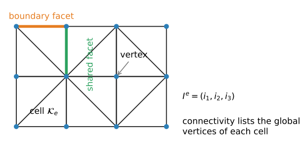
Two neighboring cells meet along a shared facet. A facet contained in \(\partial\Om\) is a boundary facet. This distinction matters because domain integrals are evaluated over cells, whereas natural boundary conditions produce integrals over boundary facets.
We also assume that the boundary mesh resolves the boundary-condition partition: every boundary facet belongs entirely to one prescribed boundary portion, such as \(\Gam_D\) or \(\Gam_N\). A change from one boundary type to another occurs only at a boundary vertex in two dimensions or along a boundary edge in three dimensions.
For later use, the size of a cell is measured by its diameter,
\[ h_e = \operatorname{diam}(\mathcal K_e) = \sup_{\bx,\bm y\in\mathcal K_e}\norm{\bx-\bm y}_2, \qquad h=\max_e h_e. \tag{6.2}\]
The number \(h\) records the largest cell size. Chapter 7 will add conditions on cell shape when it studies approximation error; those conditions are not needed for the constructions in this chapter.
For a triangular mesh, let the global mesh vertices be
\[ \bx_1,\bx_2,\ldots,\bx_{N_v}\in\R^2. \]
Each triangle has three local vertices. The connectivity map
\[ I^e:\{1,2,3\}\longrightarrow\{1,\ldots,N_v\} \tag{6.3}\]
assigns each local vertex of cell \(\mathcal K_e\) to its global vertex. If
\[ I^e=(4,7,9), \]
then local vertices 1, 2, and 3 of cell \(e\) are global vertices 4, 7, and 9. The physical coordinates of the cell are therefore
\[ \bx_1^e=\bx_4, \qquad \bx_2^e=\bx_7, \qquad \bx_3^e=\bx_9. \]
The geometry and connectivity play the same roles as in Chapter 5. The coordinates determine the physical shape of each cell; the connectivity tells us which global degrees of freedom are shared by neighboring cells.
It is useful to distinguish a vertex, which is a geometric entity of the mesh, from an interpolation node, at which a nodal degree of freedom is defined. For the linear triangular and bilinear quadrilateral elements used in this chapter, the nodes are the cell vertices. For higher-order elements, additional nodes may lie on edges, faces, or in the cell interior.
A mesh may contain many more entities than vertices and cells. In practical finite element software, facets and edges are often stored or generated because boundary conditions, interface terms, and adjacency queries require them. For the constructions below, however, the key starting data are the cell coordinates and connectivity.
Exercise 6.1 (Reading a triangular mesh) Suppose the global vertices of two triangles are numbered \(1,2,3,4\), with
\[ \bx_1=(0,0),\quad \bx_2=(1,0),\quad \bx_3=(0,1),\quad \bx_4=(1,1), \]
and the cell connectivities are
\[ I^1=(1,2,3), \qquad I^2=(2,4,3). \]
- Identify the facet shared by the two cells.
- List the boundary facets of the two-cell mesh.
- State which global vertices receive contributions from both cells.
- Explain why the shared facet is not part of the exterior boundary.
- Check whether the two cells form a conforming mesh according to the definition above.
6.2 The linear triangular element on a physical triangle
We begin with the simplest conforming two-dimensional element: a scalar linear triangular element. The cell
\[ \mathcal K_e = \operatorname{conv} \{\bx_1^e,\bx_2^e,\bx_3^e\} \]
is the convex hull of the three noncollinear vertices \(\bx_a^e=(x_a^e,y_a^e)\), \(a=1,2,3\). In this setting, the convex hull is simply the filled triangle consisting of the vertices, edges, and interior.
The local polynomial space is
\[ \mathbb P_1(\mathcal K_e) = \operatorname{span}\{1,x,y\}. \tag{6.4}\]
It has dimension three. We use the three vertex evaluations
\[ N_a(w)=w(\bx_a^e), \qquad a=1,2,3, \]
as the local degrees of freedom. In the terminology of Definition 5.1,
\[ \left( \mathcal K_e, \mathbb P_1(\mathcal K_e), \{N_1,N_2,N_3\} \right) \]
is a finite element.
As in the one-dimensional construction, we want one local basis function for each nodal degree of freedom. The basis function \(\phi_a^e\) must be linear on the triangle and satisfy
\[ \phi_a^e(\bx_b^e)=\delta_{ab}, \qquad a,b\in\{1,2,3\}. \tag{6.5}\]
A linear polynomial in two variables has the form
\[ \phi_a^e(x,y) = \alpha_a+\beta_a x+\gamma_a y. \tag{6.6}\]
The three nodal conditions determine the three coefficients. For each local basis function,
\[ \begin{bmatrix} 1 & x_1^e & y_1^e\\ 1 & x_2^e & y_2^e\\ 1 & x_3^e & y_3^e \end{bmatrix} \begin{bmatrix} \alpha_a\\ \beta_a\\ \gamma_a \end{bmatrix} = \begin{bmatrix} \delta_{a1}\\ \delta_{a2}\\ \delta_{a3} \end{bmatrix}. \tag{6.7}\]
The determinant of the matrix on the left has magnitude \(2|\mathcal K_e|\). It is therefore nonsingular when the three vertices are not collinear. The vertex values uniquely determine a function in \(\mathbb P_1(\mathcal K_e)\), so the three degrees of freedom are unisolvent.
Because \(\phi_a^e\) is linear, its gradient is constant on the cell:
\[ \grad\phi_a^e = \begin{bmatrix} \beta_a\\ \gamma_a \end{bmatrix}. \tag{6.8}\]
This is the two-dimensional analogue of the constant derivative of a one-dimensional linear shape function.
The three nodal basis functions are also called the barycentric coordinate functions of the triangle. The function \(\phi_a^e\) equals one at vertex \(a\), vanishes on the edge opposite that vertex, and varies linearly between these values. Inside the triangle,
\[ 0\le \phi_a^e\le 1, \qquad \phi_1^e+\phi_2^e+\phi_3^e=1. \tag{6.9}\]
Consequently, every point of the triangle can be written as
\[ \bx = \sum_{a=1}^{3}\phi_a^e(\bx)\bx_a^e. \tag{6.10}\]
The values \(\phi_a^e(\bx)\) are the barycentric coordinates of \(\bx\) relative to the three vertices.
6.2.1 A concrete physical triangle
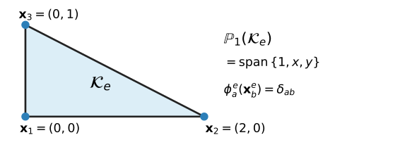
Take the triangle with vertices
\[ \bx_1=(0,0), \qquad \bx_2=(2,0), \qquad \bx_3=(0,1). \]
Solving Equation 6.7 gives
\[ \phi_1(x,y) = 1-\frac{x}{2}-y, \qquad \phi_2(x,y) = \frac{x}{2}, \qquad \phi_3(x,y) = y. \tag{6.11}\]
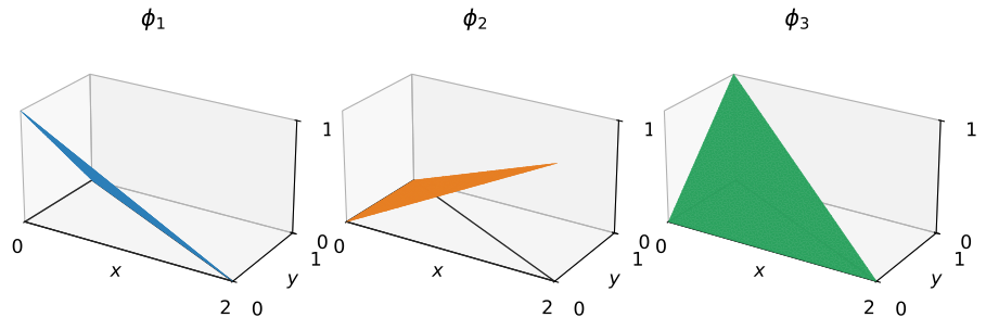
Their gradients are
\[ \grad\phi_1 = \begin{bmatrix} -1/2\\ -1 \end{bmatrix}, \qquad \grad\phi_2 = \begin{bmatrix} 1/2\\ 0 \end{bmatrix}, \qquad \grad\phi_3 = \begin{bmatrix} 0\\ 1 \end{bmatrix}. \tag{6.12}\]
For this triangle, the general partition-of-unity identity in Equation 6.9 becomes
\[ \phi_1+\phi_2+\phi_3=1. \tag{6.13}\]
For nodal values \(U_1^e,U_2^e,U_3^e\), the local finite element field is
\[ u_h|_{\mathcal K_e} = U_1^e\phi_1^e + U_2^e\phi_2^e + U_3^e\phi_3^e. \tag{6.14}\]
The nodal interpolation property gives \(u_h(\bx_a^e)=U_a^e\). Thus the interpretation of the coefficients is exactly the same as in Chapter 5.
Example 6.1 (Interpolation on the physical triangle) For the triangle in Figure 6.3, let
\[ U_1=1,\qquad U_2=3,\qquad U_3=2. \]
Using Equation 6.11,
\[ u_h(x,y) = 1\left(1-\frac{x}{2}-y\right) +3\left(\frac{x}{2}\right) +2y = 1+x+y. \]
The gradient is therefore
\[ \grad u_h = \begin{bmatrix} 1\\ 1 \end{bmatrix}. \]
The local \(P_1\) approximation is a plane over the triangle, just as the one-dimensional \(P_1\) approximation is a straight line over an interval.
Exercise 6.2 (Basis functions on a general physical triangle) For the triangle with vertices \((1,0)\), \((3,0)\), and \((2,2)\):
- solve Equation 6.7 for the three basis functions;
- verify the nodal interpolation property;
- verify that the basis functions sum to one; and
- compute their gradients;
- Identify the edge on which each basis function vanishes.
- Use Equation 6.10 to recover the point \((2,1)\) from its barycentric coordinates.
Exercise 6.3 (Reproduction of an affine function) Let
\[ p(x,y)=c_0+c_1x+c_2y \]
be any affine function, and let \(p_a=p(\bx_a^e)\) be its values at the vertices of a nondegenerate triangle. Use Equation 6.10 and the partition-of-unity property to show that
\[ p(\bx)=\sum_{a=1}^{3}p_a\phi_a^e(\bx) \]
at every point \(\bx\in\mathcal K_e\). Thus a \(P_1\) triangle reproduces every affine scalar field exactly.
6.3 From local triangles to a global conforming space
A finite element function is constructed cell by cell, but the final function must be globally admissible. For the scalar diffusion problem, the natural energy space is \(H^1(\Om)\), so the finite element field must be continuous across shared facets.
For a triangular \(P_1\) mesh, define
\[ \mathcal V_h = \left\{ v_h\in C(\overline{\Om}): v_h|_{\mathcal K_e}\in\mathbb P_1(\mathcal K_e) \text{ for every }\mathcal K_e\in\mathcal T_h \right\}. \tag{6.15}\]
One global basis function \(\phi_i\) is associated with each global mesh vertex \(\bx_i\). It satisfies
\[ \phi_i(\bx_j)=\delta_{ij} \]
and is linear on every cell. Its support is the union of the cells incident to vertex \(\bx_i\).
The local and global basis functions are related exactly as in Chapter 5:
\[ \phi_{I^e(a)}|_{\mathcal K_e} = \phi_a^e. \tag{6.16}\]
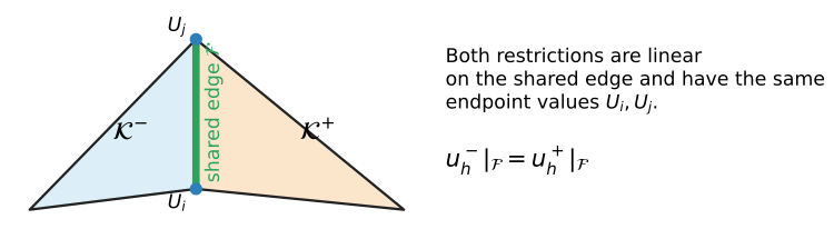
This relation explains continuity across a shared facet. Consider two triangles that share an edge with endpoints \(\bx_i\) and \(\bx_j\). The restriction of a \(P_1\) function to that edge is a one-dimensional linear polynomial. Both cells use the same nodal values at \(\bx_i\) and \(\bx_j\), so both restrictions are the same linear function along the entire shared edge. The elementwise pieces therefore join continuously.
Every \(u_h\in\mathcal V_h\) has the global representation
\[ u_h(\bx) = \sum_{j=1}^{N_v} U_j\phi_j(\bx), \tag{6.17}\]
and the nodal property again gives
\[ U_j=u_h(\bx_j). \]
The difference from one dimension is geometric rather than algebraic. A global basis function may now be supported on several triangles surrounding a vertex, and the pattern of neighboring interactions depends on the mesh connectivity.
6.4 Scalar diffusion and element equations
We now apply the multidimensional space to the scalar diffusion problem from Section 3.2.3. Let \(\Gam_D\) and \(\Gam_N\) partition the boundary, and consider
\[ -\divg(k\grad u)=f \qquad\text{in }\Om, \]
with
\[ u=g\quad\text{on }\Gam_D, \qquad k\grad u\cdot\bn=h \quad\text{on }\Gam_N. \]
The variational problem is
\[ \text{find }u\in\mathcal U_g \text{ such that}\qquad a(u,v)=\ell(v) \qquad\forall v\in\mathcal V_0, \]
where
\[ a(w,v) = \int_\Om k\,\grad w\cdot\grad v\,\dx, \]
and
\[ \ell(v) = \int_\Om f v\,\dx + \int_{\Gam_N}h v\,\ds. \tag{6.18}\]
The homogeneous finite element test space is
\[ \mathcal V_{h,0} = \mathcal V_h\cap\mathcal V_0 = \left\{ v_h\in\mathcal V_h: v_h=0\text{ on }\Gam_D \right\}. \tag{6.19}\]
To describe nonzero prescribed data, suppose \(g\) is continuous on \(\Gam_D\) and let \(g_h\) denote its nodal finite element interpolant on that boundary. The finite element trial space is
\[ \mathcal U_{h,g_h} = \left\{ w_h\in\mathcal V_h: w_h=g_h\text{ on }\Gam_D \right\}. \tag{6.20}\]
In general, \(g_h\) is an approximation of \(g\) rather than the exact boundary function. If \(g\) is itself piecewise linear on the boundary mesh, then \(g_h=g\). The discrete variational problem is
\[ \text{find }u_h\in\mathcal U_{h,g_h} \text{ such that}\qquad a(u_h,v_h)=\ell(v_h) \qquad \forall v_h\in\mathcal V_{h,0}. \tag{6.21}\]
With the global basis, \(u_h=\sum_j U_j\phi_j\). This sum includes both prescribed and unknown nodal coefficients. Testing with a basis function \(\phi_i\) associated with a free degree of freedom gives
\[ \sum_j K_{ij}U_j = F_i, \]
where
\[ K_{ij} = \int_\Om k\,\grad\phi_j\cdot\grad\phi_i\,\dx, \]
and
\[ F_i = \int_\Om f\phi_i\,\dx + \int_{\Gam_N}h\phi_i\,\ds. \tag{6.22}\]
After assembly, the terms containing prescribed coefficients are moved to the right-hand side, exactly as in Equation 5.44.
The global domain integral is decomposed cell by cell:
\[ K_{ij} = \sum_{e=1}^{N_c} \int_{\mathcal K_e} k\,\grad\phi_j\cdot\grad\phi_i\,\dx. \]
Using Equation 6.16, define the local stiffness entries
\[ K_{ab}^e = \int_{\mathcal K_e} k\, \grad\phi_b^e\cdot\grad\phi_a^e \,\dx, \tag{6.23}\]
and the local domain-load entries
\[ F_a^e = \int_{\mathcal K_e} f\,\phi_a^e\,\dx. \tag{6.24}\]
Natural boundary data contribute through boundary facets. If a facet \(\mathcal F\subset\partial\mathcal K_e\cap\Gam_N\), its contribution is
\[ F_a^{\mathcal F} = \int_{\mathcal F} h\,\phi_a^e\,\ds. \tag{6.25}\]
To evaluate this integral, map the reference interval \(\widehat{\mathcal F}=[-1,1]\) to the straight physical edge with endpoints \(\bx_i\) and \(\bx_j\):
\[ \bx(\zeta) = \frac{1-\zeta}{2}\bx_i + \frac{1+\zeta}{2}\bx_j. \tag{6.26}\]
The edge Jacobian is the length of the tangent vector,
\[ J_{\mathcal F} = \norm{\frac{\dd\bx}{\dd\zeta}}_2 = \frac{\norm{\bx_j-\bx_i}_2}{2} = \frac{L_{\mathcal F}}{2}. \tag{6.27}\]
Therefore,
\[ \int_{\mathcal F}h\,\phi_a^e\,\ds = \int_{-1}^{1} h(\bx(\zeta)) \widehat\phi_a(\zeta) J_{\mathcal F} \,\dd\zeta. \tag{6.28}\]
This is an ordinary one-dimensional integral on the reference edge.
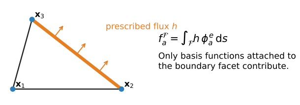
The global load vector therefore receives contributions from both cells and boundary facets.
Example 6.2 (Element matrix for the concrete triangle) For the triangle in Figure 6.3, the area is
\[ |\mathcal K_e|=1. \]
If \(k\) is constant on the cell, the basis gradients in Equation 6.12 are constant, so
\[ K_{ab}^e = k|\mathcal K_e| \grad\phi_b^e\cdot\grad\phi_a^e. \]
Hence
\[ \bK^e = k \begin{bmatrix} 5/4 & -1/4 & -1\\ -1/4 & 1/4 & 0\\ -1 & 0 & 1 \end{bmatrix}. \tag{6.29}\]
If the source \(f\) is constant, each linear basis function has average value \(1/3\) over the triangle. Therefore
\[ \bF^e = \frac{f|\mathcal K_e|}{3} \begin{bmatrix} 1\\ 1\\ 1 \end{bmatrix} = \frac{f}{3} \begin{bmatrix} 1\\ 1\\ 1 \end{bmatrix}. \tag{6.30}\]
As in one dimension,
\[ \bK^e \begin{bmatrix} 1\\ 1\\ 1 \end{bmatrix} = \bm{0}, \]
because a constant nodal field has zero gradient.
Example 6.3 (A constant flux on one edge) Let a boundary edge of a \(P_1\) triangle have length \(L_{\mathcal F}\) and let the prescribed normal flux be the constant \(h_0\). Only the two vertex basis functions associated with the edge are nonzero on that facet. Their restrictions are \((1-\zeta)/2\) and \((1+\zeta)/2\). Using Equation 6.28 gives
\[ \int_{\mathcal F}h_0\phi_i^e\,\ds = \frac{h_0L_{\mathcal F}}{2} \int_{-1}^{1}\frac{1-\zeta}{2}\,\dd\zeta = \frac{h_0L_{\mathcal F}}{2}, \]
and the same value is obtained for the other endpoint. Hence the facet load vector is
\[ \bF^{\mathcal F} = \frac{h_0L_{\mathcal F}}{2} \begin{bmatrix} 1\\ 1 \end{bmatrix}. \]
These two entries are assembled into the global load vector at the two global vertices of the boundary edge.
Exercise 6.5 (A linearly varying boundary flux) On a straight edge of length \(L_{\mathcal F}\), let the prescribed flux vary linearly from \(h_i\) at endpoint \(i\) to \(h_j\) at endpoint \(j\).
- Express \(h(\zeta)\) using the two linear reference-edge basis functions.
- Use Equation 6.28 to derive the two-entry consistent facet load vector.
- Verify that the sum of its entries equals \(L_{\mathcal F}(h_i+h_j)/2\), the integral of the prescribed flux over the edge.
Exercise 6.6 (A \(P_1\) diffusion element) For the triangle with vertices \((0,0)\), \((1,0)\), and \((0,1)\):
- derive the three basis functions;
- compute their gradients;
- derive the element stiffness matrix for constant \(k\);
- derive the element load vector for constant \(f\); and
- verify that the row sums of the stiffness matrix are zero.
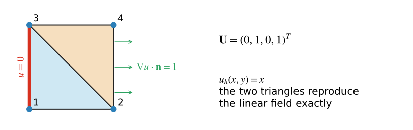
Example 6.4 (Assembly and solution on two triangles) Consider the unit square with vertices
\[ \bx_1=(0,0),\quad \bx_2=(1,0),\quad \bx_3=(0,1),\quad \bx_4=(1,1), \]
and triangle connectivities
\[ I^1=(1,2,3), \qquad I^2=(2,4,3). \]
Let \(k=1\) and \(f=0\). Prescribe \(u=0\) on the left boundary, \(\grad u\cdot\bn=1\) on the right boundary, and zero normal flux on the top and bottom boundaries.
Direct calculation gives
\[ \bK^1 = \frac12 \begin{bmatrix} 2&-1&-1\\ -1&1&0\\ -1&0&1 \end{bmatrix}, \qquad \bK^2 = \frac12 \begin{bmatrix} 1&-1&0\\ -1&2&-1\\ 0&-1&1 \end{bmatrix}. \]
Scatter-adding these matrices with the two connectivity maps produces
\[ \bK = \begin{bmatrix} 1&-1/2&-1/2&0\\ -1/2&1&0&-1/2\\ -1/2&0&1&-1/2\\ 0&-1/2&-1/2&1 \end{bmatrix}. \tag{6.31}\]
The right boundary edge has length one, so the constant-flux calculation in Example 6.3 gives
\[ \bF = \begin{bmatrix} 0&1/2&0&1/2 \end{bmatrix}^T. \]
The entries are ordered by global vertices \(1,2,3,4\).
The prescribed coefficients are \(U_1=U_3=0\). The equations for the two free coefficients are
\[ \begin{bmatrix} 1&-1/2\\ -1/2&1 \end{bmatrix} \begin{bmatrix} U_2\\U_4 \end{bmatrix} = \begin{bmatrix} 1/2\\1/2 \end{bmatrix}, \]
which gives \(U_2=U_4=1\). Therefore the assembled finite element field is \(u_h(x,y)=x\) on both triangles. This linear field satisfies the differential equation and all four boundary conditions, so the two-element mesh reproduces the exact solution.
Exercise 6.7 (Reusing the two-triangle mesh) On the mesh in Example 6.4, set \(k=1\), \(f=1\), prescribe \(u=0\) on the left boundary, and prescribe zero normal flux elsewhere.
- Derive the element load vector on each triangle.
- Assemble the global load vector.
- Solve the two-by-two reduced system for \(U_2\) and \(U_4\).
- Write the resulting piecewise-linear function separately on each triangle.
6.5 Reference triangles and coordinate mappings
The physical-triangle construction shows exactly what the basis functions mean, but an implementation should not solve a new interpolation system on every cell. As in Chapter 5, we define basis functions once on a reference cell and map them to the physical cells.
For triangles, use the reference cell
\[ \widehat{\mathcal K} = \left\{ (\xi,\eta): \xi\ge0,\ \eta\ge0,\ \xi+\eta\le1 \right\}, \tag{6.32}\]
with reference vertices
\[ \widehat{\bx}_1=(0,0), \qquad \widehat{\bx}_2=(1,0), \qquad \widehat{\bx}_3=(0,1). \]
We collect the reference coordinates as
\[ \bm{\xi} = \begin{bmatrix}\xi&\eta\end{bmatrix}^T. \]
The reference \(P_1\) basis functions are
\[ \widehat\phi_1(\xi,\eta) = 1-\xi-\eta, \qquad \widehat\phi_2(\xi,\eta) = \xi, \qquad \widehat\phi_3(\xi,\eta) = \eta. \tag{6.33}\]
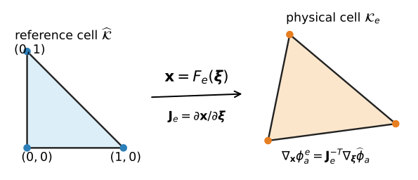
For the physical triangle with vertices \(\bx_1^e,\bx_2^e,\bx_3^e\), define the affine map
\[ \bx = F_e(\bm{\xi}) = \bx_1^e + \bm{J}_e \begin{bmatrix} \xi\\ \eta \end{bmatrix}, \tag{6.34}\]
where
\[ \bm{J}_e = \begin{bmatrix} x_2^e-x_1^e & x_3^e-x_1^e\\ y_2^e-y_1^e & y_3^e-y_1^e \end{bmatrix}. \tag{6.35}\]
The two columns of \(\bm J_e\) are the physical edge vectors from local vertex 1 to local vertices 2 and 3.
The determinant measures the change in area:
\[ \dd x = |\det\bm J_e|\, \dd\bm{\xi}, \tag{6.36}\]
where \(\dd\bm{\xi}=\dd\xi\,\dd\eta\). Since the reference triangle has area \(1/2\),
\[ |\mathcal K_e| = \frac12|\det\bm J_e|. \tag{6.37}\]
A valid affine triangle map requires \(\det\bm J_e\ne0\). In a consistently oriented mesh, the local vertex ordering is usually chosen so that \(\det\bm J_e>0\). In two dimensions this is obtained by listing the three local vertices counterclockwise.
6.5.1 Transformation of gradients
The physical basis function is
\[ \phi_a^e(\bx) = \widehat\phi_a(F_e^{-1}(\bx)). \]
The gradient transformation follows from the chain rule. Since
\[ \widehat\phi_a(\bm{\xi}) = \phi_a^e(F_e(\bm{\xi})), \]
differentiation with respect to the reference coordinate gives
\[ \grad_{\bm{\xi}}\widehat\phi_a = \bm J_e^T \grad_{\bx}\phi_a^e. \]
Therefore,
\[ \boxed{ \grad_{\bx}\phi_a^e = \bm J_e^{-T} \grad_{\bm{\xi}}\widehat\phi_a. } \tag{6.38}\]
This formula is the multidimensional counterpart of the one-dimensional factor \(1/J_e\) in Chapter 5. The difference is that the Jacobian is now a matrix and the gradient is a vector.
For a two-dimensional triangle, \(\bm J_e\in\R^{2\times2}\), \(\grad_{\bm{\xi}}\widehat\phi_a\in\R^2\), and \(\grad_{\bx}\phi_a^e\in\R^2\). The inverse transpose follows directly from solving the chain-rule relation \(\grad_{\bm{\xi}}\widehat\phi_a=\bm J_e^T\grad_{\bx}\phi_a^e\) for the physical gradient.
Example 6.5 (Mapping the concrete triangle) For the physical triangle with vertices \((0,0)\), \((2,0)\), and \((0,1)\),
\[ \bm J_e = \begin{bmatrix} 2&0\\ 0&1 \end{bmatrix}, \qquad \det\bm J_e=2. \]
Hence \(|\mathcal K_e|=\tfrac12(2)=1\), as used previously. Moreover,
\[ \grad_{\bx}\phi_a^e = \begin{bmatrix} 1/2&0\\ 0&1 \end{bmatrix} \grad_{\bm{\xi}}\widehat\phi_a, \]
which recovers the physical gradients in Equation 6.12.
Exercise 6.8 (Checking the gradient transformation) For a physical triangle with vertices \((1,1)\), \((4,1)\), and \((2,3)\):
- form \(\bm J_e\) and compute its determinant;
- calculate the physical area;
- compute \(\bm J_e^{-T}\);
- transform the three reference gradients; and
- construct the physical basis functions \(\phi_a^e=\widehat\phi_a\circ F_e^{-1}\) and verify that their directly computed gradients agree with the transformed gradients from Part 4.
6.6 Multidimensional quadrature and boundary integration
After transformation to a reference cell, a typical element integral has the form
\[ \int_{\mathcal K_e} g(\bx)\,\dx = \int_{\widehat{\mathcal K}} g(F_e(\bm{\xi})) |\det\bm J_e(\bm{\xi})| \,\dd\bm{\xi}. \tag{6.39}\]
For affine triangles, \(\bm J_e\) is constant. For more general isoparametric cells, the Jacobian may vary across the cell.
A quadrature rule on the reference triangle approximates
\[ \int_{\widehat{\mathcal K}} g(\xi,\eta)\,\dd\xi\,\dd\eta \approx \sum_{q=1}^{n_q} w_qg(\xi_q,\eta_q). \tag{6.40}\]
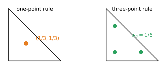
For the reference triangle in Equation 6.32, useful low-order rules include:
| rule | points | weights | polynomial exactness |
|---|---|---|---|
| one point | \((1/3,1/3)\) | \(1/2\) | degree 1 |
| three point | \((1/6,1/6)\), \((2/3,1/6)\), \((1/6,2/3)\) | \(1/6\) each | degree 2 |
The weights sum to \(1/2\), the area of the reference triangle.
The transformed scalar-diffusion stiffness entry is
\[ K_{ab}^e = \int_{\widehat{\mathcal K}} k(F_e(\bm{\xi})) \left( \bm J_e^{-T} \grad_{\bm{\xi}}\widehat\phi_b \right) \cdot \left( \bm J_e^{-T} \grad_{\bm{\xi}}\widehat\phi_a \right) |\det\bm J_e| \,\dd\bm{\xi}. \tag{6.41}\]
For a \(P_1\) affine triangle with constant \(k\), the physical gradients and the Jacobian are constant, so the stiffness integrand is constant. A one-point rule is therefore sufficient. More complicated coefficients, higher-order basis functions, or nonaffine geometry may require higher-order quadrature.
For example, the element load entry is approximated by
\[ F_a^e \approx \sum_{q=1}^{n_q} w_q f(F_e(\bm\xi_q)) \widehat\phi_a(\bm\xi_q) |\det\bm J_e(\bm\xi_q)|. \tag{6.42}\]
For constant \(f\) on an affine \(P_1\) triangle, the integrand is linear. The one-point rule gives
\[ F_a^e = \frac12 f\frac13|\det\bm J_e| = \frac{f|\mathcal K_e|}{3}, \]
which agrees with Equation 6.30.
Boundary-facet integrals are transformed separately. In two dimensions a facet is a line segment, so the one-dimensional quadrature rules from Chapter 5 can be reused on a reference edge. In three dimensions a facet is a two-dimensional surface and requires a surface quadrature rule.
Exercise 6.9 (Triangle quadrature)
- Verify that the one-point rule integrates the three reference basis functions exactly.
- Verify that the three-point rule integrates \(\xi^2\), \(\xi\eta\), and \(\eta^2\) exactly.
- Explain why the one-point rule is sufficient for the stiffness matrix of a \(P_1\) affine triangle with constant diffusivity.
- Determine whether the one-point rule exactly evaluates the load vector when \(f(x,y)=x+y\) and the geometry map is affine.
6.7 Quadrilateral cells
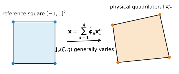
An affine map sends the reference triangle to any physical triangle. A general four-sided cell requires a different construction because an affine map can produce only a parallelogram. The standard four-node quadrilateral begins with the reference square
\[ \widehat{\mathcal K}=[-1,1]^2 \]
and the tensor-product polynomial space
\[ \mathbb Q_1(\widehat{\mathcal K}) = \operatorname{span}\{1,\xi,\eta,\xi\eta\}. \tag{6.43}\]
The notation \(\mathbb Q_1\) means that the polynomial degree is at most one in each coordinate separately. The product \(\xi\eta\) is therefore included even though its total degree is two. The four local nodes are ordered
\[ (-1,-1),\qquad (1,-1),\qquad (1,1),\qquad (-1,1), \]
and the corresponding nodal basis functions are
\[ \begin{aligned} \widehat\phi_1(\xi,\eta) &=\frac14(1-\xi)(1-\eta),& \widehat\phi_2(\xi,\eta) &=\frac14(1+\xi)(1-\eta),\\ \widehat\phi_3(\xi,\eta) &=\frac14(1+\xi)(1+\eta),& \widehat\phi_4(\xi,\eta) &=\frac14(1-\xi)(1+\eta). \end{aligned} \tag{6.44}\]
They satisfy the nodal interpolation property and sum to one. Each restriction to a reference edge is a one-dimensional linear function.
6.7.1 Isoparametric geometry and field interpolation
The geometry map is defined by
\[ \bx = F_e(\xi,\eta) = \sum_{a=1}^{4} \widehat\phi_a(\xi,\eta)\bx_a^e. \tag{6.45}\]
The same reference functions are used to interpolate the finite element field,
\[ u_h(F_e(\xi,\eta)) = \sum_{a=1}^{4} U_a^e\widehat\phi_a(\xi,\eta). \tag{6.46}\]
Using the same basis for the geometry and the field is the isoparametric construction introduced in Chapter 5.
The physical basis is again obtained by composition,
\[ \phi_a^e(\bx) = \widehat\phi_a(F_e^{-1}(\bx)). \]
For a general quadrilateral, the Jacobian matrix
\[ \bm J_e(\xi,\eta) = \begin{bmatrix} \partial x/\partial\xi&\partial x/\partial\eta\\ \partial y/\partial\xi&\partial y/\partial\eta \end{bmatrix} \tag{6.47}\]
varies across the cell. Consequently, \(\bm J_e^{-T}\) and \(|\det\bm J_e|\) must be evaluated at every quadrature point. A valid, orientation-preserving element must satisfy
\[ \det\bm J_e(\xi,\eta)>0 \qquad \text{throughout }\widehat{\mathcal K}. \tag{6.48}\]
If the physical cell is a parallelogram, the map reduces to an affine map and \(\bm J_e\) is constant. For a non-parallelogram, the map is bilinear and the mapped basis functions are generally not polynomials in the physical coordinates \((x,y)\).
Example 6.6 (Jacobian of a nonrectangular quadrilateral) Consider the physical vertices
\[ \bx_1=(0,0),\quad \bx_2=(2,0),\quad \bx_3=(5/2,1),\quad \bx_4=(0,1). \]
Substitution into Equation 6.45 gives
\[ x(\xi,\eta) = (1+\xi)\left(\frac98+\frac18\eta\right), \qquad y(\xi,\eta)=\frac{1+\eta}{2}. \]
Therefore,
\[ \bm J_e(\xi,\eta) = \begin{bmatrix} 9/8+\eta/8&(1+\xi)/8\\ 0&1/2 \end{bmatrix}, \qquad \det\bm J_e = \frac{9+\eta}{16}. \tag{6.49}\]
The determinant varies between \(1/2\) and \(5/8\) on the reference square and is positive everywhere. The mapping is valid, but geometric factors must be recomputed at each quadrature point.
A tensor-product Gauss rule is natural on the reference square. A \(2\times2\) rule uses the four combinations
\[ (\xi_q,\eta_q) \in \left\{-\frac1{\sqrt3},\frac1{\sqrt3}\right\} \times \left\{-\frac1{\sqrt3},\frac1{\sqrt3}\right\}, \tag{6.50}\]
with unit weights. At each point, the implementation evaluates the reference basis, \(\bm J_e\), \(\det\bm J_e\), the transformed gradients, and the integrand.
Exercise 6.10 (Properties and integration of a \(Q_1\) element)
- Verify the nodal interpolation and partition-of-unity properties of
- Show that the restriction of the four basis functions to each reference edge is linear.
- For the element in Example 6.6, evaluate \(F_e\), \(\bm J_e\), and \(\det\bm J_e\) at the four points in Equation 6.50.
- Map the four Gauss points to the physical element.
- Explain why one constant Jacobian cannot be used for this element.
6.8 Tetrahedral cells
The three-dimensional analogue of a triangle is a tetrahedron. The reference tetrahedron is
\[ \widehat{\mathcal K} = \left\{(\xi,\eta,\zeta): \xi,\eta,\zeta\ge0, \ \xi+\eta+\zeta\le1 \right\}. \tag{6.51}\]
Its four vertices are the origin and the three Cartesian unit vectors. The \(P_1\) nodal basis is
\[ \widehat\phi_1=1-\xi-\eta-\zeta, \qquad \widehat\phi_2=\xi, \qquad \widehat\phi_3=\eta, \qquad \widehat\phi_4=\zeta. \tag{6.52}\]
In this subsection the reference-coordinate vector is
\[ \bm\xi = \begin{bmatrix}\xi&\eta&\zeta\end{bmatrix}^T. \]
For physical vertices \(\bx_1^e,\ldots,\bx_4^e\), the affine map is
\[ F_e(\bm\xi) = \bx_1^e + \bm J_e \begin{bmatrix}\xi\\\eta\\\zeta\end{bmatrix}, \qquad \bm J_e = \begin{bmatrix} \bx_2^e-\bx_1^e& \bx_3^e-\bx_1^e& \bx_4^e-\bx_1^e \end{bmatrix}. \tag{6.53}\]
The reference tetrahedron has volume \(1/6\), so
\[ |\mathcal K_e| = \frac{|\det\bm J_e|}{6}. \tag{6.54}\]
With a consistent orientation, the local vertex ordering is chosen so that \(\det\bm J_e>0\).
The volume and gradient transformations have exactly the same form as in two dimensions:
\[ \dx=|\det\bm J_e|\,\dd\bm\xi, \qquad \grad_{\bx}\phi_a^e = \bm J_e^{-T}\grad_{\bm\xi}\widehat\phi_a. \]
The centroid rule evaluates the integrand at
\[ \bm\xi_q = \begin{bmatrix}1/4&1/4&1/4\end{bmatrix}^T \]
with weight \(w_q=1/6\). It integrates every polynomial of total degree at most one exactly on the reference tetrahedron.
Exercise 6.11 (A physical tetrahedron) Consider the tetrahedron with vertices
\[ (0,0,0),\qquad(2,0,0),\qquad(0,1,0),\qquad(0,0,3). \]
- Form \(\bm J_e\) and compute the physical volume.
- Compute the four physical basis gradients.
- Verify that the gradients sum to zero.
- For constant \(k\), write the \(4\times4\) element stiffness matrix in the form \(K_{ab}^e=k|\mathcal K_e|\grad\phi_b^e\cdot\grad\phi_a^e\).
6.9 Hexahedral cells
A hexahedron is the three-dimensional tensor-product analogue of a quadrilateral. On the reference cube \([-1,1]^3\), associate each vertex with a sign triple \((\xi_a,\eta_a,\zeta_a)\in\{-1,1\}^3\). The eight trilinear basis functions can be written compactly as
\[ \widehat\phi_a(\xi,\eta,\zeta) = \frac18 (1+\xi_a\xi) (1+\eta_a\eta) (1+\zeta_a\zeta), \qquad a=1,\ldots,8. \tag{6.55}\]
Their span is
\[ \mathbb Q_1 = \operatorname{span} \{1,\xi,\eta,\zeta,\xi\eta,\xi\zeta,\eta\zeta,\xi\eta\zeta\}. \]
The geometry map \(\bx=\sum_a\widehat\phi_a\bx_a^e\) is trilinear, and a general physical hexahedron has a Jacobian that varies within the cell. Volume integrals use
\[ \int_{\mathcal K_e}g(\bx)\,\dx = \int_{[-1,1]^3} g(F_e(\bm\xi))|\det\bm J_e(\bm\xi)|\,\dd\bm\xi. \]
A valid orientation-preserving hexahedral map must satisfy \(\det\bm J_e(\bm\xi)>0\) throughout the reference cube.
Tensor-product Gauss quadrature forms the three-dimensional quadrature points from one-dimensional Gauss points. The same sequence—map points, evaluate the Jacobian, transform gradients, and accumulate local arrays—therefore applies to triangles, quadrilaterals, tetrahedra, and hexahedra.
Exercise 6.12 (The reference \(Q_1\) hexahedron)
- Verify the nodal property of Equation 6.55 at the eight sign triples.
- Verify that the eight functions sum to one.
- How many points are produced by a \(2\times2\times2\) tensor-product Gauss rule?
- Explain why the Jacobian is constant for an affine parallelepiped, including a rectangular box, but may vary for a general distorted hexahedron.
6.10 Vector-valued approximation and linear elasticity
The scalar construction extends naturally to vector-valued fields. In two-dimensional elasticity, the displacement has two components,
\[ \bu(\bx) = \begin{bmatrix} u_1(\bx)\\ u_2(\bx) \end{bmatrix}, \]
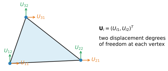
so each nodal vertex of a displacement-based element carries two displacement degrees of freedom.
Let \(\mathcal V_h\) be the scalar finite element space. Its vector-valued counterpart is
\[ \mathcal V_h(\Om;\R^2) = \left\{ \bm w_h:\Om\to\R^2: w_{h1},w_{h2}\in\mathcal V_h \right\}. \tag{6.56}\]
Using the displacement boundary data from Equation 4.34, define
\[ \begin{aligned} \mathcal U_{h,\overline{\bu}_h} &=\{\bm w_h\in\mathcal V_h(\Om;\R^2): \bm w_h=\overline{\bu}_h\text{ on }\Gam_u\},\\ \mathcal V_{h,0} &=\{\bv_h\in\mathcal V_h(\Om;\R^2): \bv_h=\bm 0\text{ on }\Gam_u\}. \end{aligned} \tag{6.57}\]
Here \(\overline{\bu}_h\) is the finite element interpolation of the prescribed boundary displacement. The discrete elasticity problem is the restriction of Equation 4.36 to these spaces:
\[ \left. \begin{aligned} &\text{Find }\bu_h\in\mathcal U_{h,\overline{\bu}_h}\text{ such that}\\ &\int_{\Om} \beps(\bv_h):\mathbb C:\beps(\bu_h)\,\dx = \int_{\Om}\rho\bb\cdot\bv_h\,\dx + \int_{\Gam_t}\overline{\bt}\cdot\bv_h\,\ds \quad\forall\bv_h\in\mathcal V_{h,0}. \end{aligned} \right\} \qquad\text{Discrete variational problem} \tag{6.58}\]
Using the scalar basis functions \(\phi_i\), write
\[ \bu_h(\bx) = \sum_i \phi_i(\bx)\bm U_i, \qquad \bm U_i = \begin{bmatrix} U_{i1}\\ U_{i2} \end{bmatrix}. \tag{6.59}\]
On one three-node triangle,
\[ \bu_h|_{\mathcal K_e} = \sum_{a=1}^{3} \phi_a^e\bm U_a^e. \]
Collect the six element coefficients as
\[ \bU^e = \begin{bmatrix} U_{11}^e& U_{12}^e& U_{21}^e& U_{22}^e& U_{31}^e& U_{32}^e \end{bmatrix}^T. \]
The ordering is by vertex: the two components at vertex 1 are followed by the two components at vertex 2 and then those at vertex 3. Other orderings are possible, but the element degree-of-freedom map and every element matrix must use the same ordering.
Then
\[ \bu_h|_{\mathcal K_e} = \bN^e\bU^e, \]
with
\[ \bN^e = \begin{bmatrix} \phi_1^e&0&\phi_2^e&0&\phi_3^e&0\\ 0&\phi_1^e&0&\phi_2^e&0&\phi_3^e \end{bmatrix}. \tag{6.60}\]
Using the engineering-strain ordering in Equation 4.27,
\[ \beps_{\mathrm V} = \begin{bmatrix} \varepsilon_{11}\\ \varepsilon_{22}\\ \gamma_{12} \end{bmatrix}, \]
the element strain is
\[ \beps_{\mathrm V} = \bB^e\bU^e, \]
where
\[ \bB^e = \begin{bmatrix} \phi_{1,x}^e&0& \phi_{2,x}^e&0& \phi_{3,x}^e&0\\ 0&\phi_{1,y}^e& 0&\phi_{2,y}^e& 0&\phi_{3,y}^e\\ \phi_{1,y}^e&\phi_{1,x}^e& \phi_{2,y}^e&\phi_{2,x}^e& \phi_{3,y}^e&\phi_{3,x}^e \end{bmatrix}. \tag{6.61}\]
For a \(P_1\) triangle, the basis gradients are constant, so \(\bB^e\) is constant on the cell. This is the familiar constant-strain triangle.
Let \(\bm C_{\mathrm V}\) be the plane-stress or plane-strain constitutive matrix consistent with Equation 4.30. The element stiffness matrix is
\[ \bK^e = \int_{\mathcal K_e} (\bB^e)^T \bm C_{\mathrm V} \bB^e \,\dx. \tag{6.62}\]
The body-force and traction contributions are
\[ \bF^e = \int_{\mathcal K_e} (\bN^e)^T\rho\bb\,\dx + \int_{\partial\mathcal K_e\cap\Gam_t} (\bN^e)^T\overline{\bt}\,\ds. \tag{6.63}\]
These two-dimensional formulas are written per unit out-of-plane thickness. If the model represents a body with constant thickness \(t\), both the domain and edge contributions are multiplied by \(t\).
The mathematical pattern is the same as for scalar diffusion: basis functions define the approximation, derivatives form the element strain or gradient operator, element integrals produce local arrays, and connectivity determines where those arrays enter the global system.
Example 6.7 (Strain in a constant-strain triangle) For the triangle in Figure 6.3, the basis gradients in Equation 6.12 give
\[ \bB^e = \begin{bmatrix} -1/2&0&1/2&0&0&0\\ 0&-1&0&0&0&1\\ -1&-1/2&0&1/2&1&0 \end{bmatrix}. \tag{6.64}\]
Consider the affine displacement field
\[ \bu(x,y) = \begin{bmatrix} 2x+y\\ -x+3y \end{bmatrix}. \]
Its nodal coefficient vector is
\[ \bU^e = \begin{bmatrix} 0&0&4&-2&1&3 \end{bmatrix}^T. \]
Multiplication by Equation 6.64 gives
\[ \beps_{\mathrm V} = \bB^e\bU^e = \begin{bmatrix} 2\\3\\0 \end{bmatrix}. \]
The first two entries are \(\varepsilon_{11}\) and \(\varepsilon_{22}\). The third is the engineering shear strain \(\gamma_{12}=u_{1,2}+u_{2,1}=1-1=0\). Because the element reproduces affine displacements, it reproduces their constant strains exactly.
Exercise 6.13 (Rigid motions and the constant-strain triangle) Use Equation 6.64 to verify the following statements.
- If every node is given the same translation \((c_1,c_2)^T\), then \(\bB^e\bU^e=\bm 0\).
- The infinitesimal rigid rotation \(\bu(x,y)=(-\theta y,\theta x)^T\) also gives \(\bB^e\bU^e=\bm 0\).
- Explain why these results are required of a physically meaningful linear elastic element.
Exercise 6.14 (Local and global displacement degrees of freedom) A two-dimensional triangular mesh has global vertices \(1,2,3,4\) and cells
\[ I^1=(1,2,3), \qquad I^2=(2,4,3). \]
Assume two displacement components per vertex.
- Give one consistent global numbering of the eight displacement degrees of freedom.
- Write the six global degree-of-freedom numbers associated with each cell.
- Identify which displacement degrees of freedom are shared by the two triangles.
- Explain how the scalar vertex connectivity is expanded into a vector-valued degree-of-freedom map.
6.11 Assembly and essential boundary conditions
For scalar \(P_1\) diffusion, each triangular cell has three local degrees of freedom. For two-dimensional displacement elasticity, the same triangle has six. The local-to-global assembly rule itself is unchanged.
If local scalar indices \(a,b\) correspond to global indices \(I^e(a),I^e(b)\),
\[ K_{I^e(a),I^e(b)} \mathrel{+}= K_{ab}^e, \qquad F_{I^e(a)} \mathrel{+}= F_a^e. \tag{6.65}\]
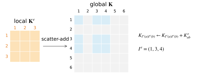
For vector-valued elements, the element degree-of-freedom map replaces the vertex map in this rule. A vertex shared by several cells contributes the same global displacement components to each incident cell.
The global stiffness matrix remains sparse because a basis function interacts only with basis functions supported on cells that overlap its support. In two and three dimensions, the sparsity pattern is no longer a simple narrow band under arbitrary numbering, but it still reflects mesh adjacency.
Essential boundary conditions are imposed on global degrees of freedom associated with the prescribed boundary. The same partitioning from Chapter 5 applies:
\[ \bK_{ff}\bU_f = \bF_f-\bK_{fp}\bU_p. \tag{6.66}\]
The geometric task is more involved because a boundary condition is usually specified on a boundary portion rather than at a single endpoint. The mesh must therefore identify the boundary facets belonging to \(\Gam_D\) or \(\Gam_u\), and the finite element software must identify the degrees of freedom attached to those facets.
Natural boundary conditions require the same boundary-facet identification, but their contribution is assembled into the load vector through facet integrals rather than through prescribed coefficient values.
6.12 Connection to FEniCSx
The mathematical construction above corresponds closely to the objects used by FEniCSx. The software automates reference-cell evaluation, coordinate mapping, quadrature, degree-of-freedom maps, local element kernels, and sparse assembly, but the objects being manipulated are the same ones developed in this chapter. The theory in Chapters 5 and 6 uses one-based numbering. Python arrays and FEniCSx degree-of-freedom maps use zero-based indices, so mathematical index \(i\) is represented by Python index i - 1 when these objects are stored in code. Accordingly, x[0] in the example below denotes the first spatial coordinate.
| Mathematical object | FEniCSx counterpart |
|---|---|
| mesh \(\mathcal T_h\) | dolfinx.mesh.Mesh |
| cell type and geometry | mesh topology and geometry |
| finite element space \(\mathcal V_h\) | fem.functionspace(...) |
| trial and test functions | ufl.TrialFunction, ufl.TestFunction |
| gradient and inner products | UFL grad, inner |
| domain integral | ufl.dx |
| boundary-facet integral | ufl.ds |
| Dirichlet degrees of freedom | fem.locate_dofs_* |
| essential boundary condition | fem.dirichletbc |
| assembled linear problem | dolfinx.fem.petsc.LinearProblem |
A minimal scalar-diffusion example on a triangular mesh is:
import numpy as np
import ufl
from mpi4py import MPI
from petsc4py import PETSc
from dolfinx import fem, mesh
from dolfinx.fem.petsc import LinearProblem

domain = mesh.create_unit_square(
    MPI.COMM_WORLD, 16, 16, cell_type=mesh.CellType.triangle
)

V = fem.functionspace(domain, ("Lagrange", 1))

u = ufl.TrialFunction(V)
v = ufl.TestFunction(V)

k = fem.Constant(domain, PETSc.ScalarType(1.0))
f = fem.Constant(domain, PETSc.ScalarType(1.0))

a = k * ufl.inner(ufl.grad(u), ufl.grad(v)) * ufl.dx
L = f * v * ufl.dx

fdim = domain.topology.dim - 1
left_facets = mesh.locate_entities_boundary(
    domain, fdim, lambda x: np.isclose(x[0], 0.0)
)
left_dofs = fem.locate_dofs_topological(V, fdim, left_facets)

bc = fem.dirichletbc(PETSc.ScalarType(0.0), left_dofs, V)

problem = LinearProblem(
    a,
    L,
    bcs=[bc],
    petsc_options_prefix="diffusion_",
    petsc_options={"ksp_type": "preonly", "pc_type": "lu"},
)

u_h = problem.solve()

# The exact solution is u(x, y) = x - x^2/2.
x = ufl.SpatialCoordinate(domain)
u_exact = x[0] - 0.5 * x[0] ** 2
error_form = fem.form((u_h - u_exact) ** 2 * ufl.dx)
error_local = fem.assemble_scalar(error_form)
error_L2 = np.sqrt(domain.comm.allreduce(error_local, op=MPI.SUM))

if domain.comm.rank == 0:
    print(f"L2 error: {error_L2:.6e}")
The exact solution satisfies
\[ -\Delta u=1, \qquad u=0\text{ on }x=0, \qquad \grad u\cdot\bn=0 \text{ on the remaining boundary}. \]
The code therefore checks the computed field against the boundary-value problem it solves rather than reporting a solution with no verification.
The UFL expression
k * ufl.inner(ufl.grad(u), ufl.grad(v)) * ufl.dxrepresents the same bilinear form as
\[ \int_\Om k\,\grad u_h\cdot\grad v_h\,\dx. \]
FEniCSx evaluates this form cell by cell, transforms basis gradients from reference to physical coordinates, applies quadrature, and assembles the local contributions into a global PETSc matrix. The code does not replace the derivation; it implements it.
Boundary integrals are introduced by adding terms with ufl.ds. Vector-valued elasticity uses a vector function space and the strain operator \(\operatorname{sym}\grad\bu\) from Chapter 4. The same mesh, mapping, quadrature, and assembly concepts remain in place.
Exercise 6.15 (Verifying the FEniCSx solution) For the code above:
- Identify the mesh, finite element space, trial function, test function, bilinear form, linear functional, and prescribed boundary condition in the code.
- Run the calculation with \(8\times8\), \(16\times16\), and \(32\times32\) subdivisions and record the \(L^2\) error.
- Confirm that the error decreases as the mesh is refined.
- Change the finite element degree from one to two, repeat the calculation, and compare the errors on the same meshes. Before running the code, predict the result: \(u=x-x^2/2\) belongs to the quadratic finite element space on this affine triangular mesh. Relate the observed error to the exact representation in Example 5.6.
- Explain which steps of the element loop in Section 6.13 are carried out internally by FEniCSx.
6.13 A complete multidimensional finite element procedure
The multidimensional finite element method can now be organized as the same local-to-global procedure used in one dimension, with additional geometric transformations.
read the mesh coordinates, cell connectivity, and boundary tags
choose the finite element and quadrature rules
initialize the global matrix K and vector F

for each cell e:
    read the cell coordinates and global degree-of-freedom map
    initialize the element matrix K_e and domain-load vector f_e

    for each cell quadrature point q:
        evaluate reference basis functions and reference gradients
        map the quadrature point to the physical cell
        evaluate J_e, det(J_e), and J_e^{-T}
        transform the basis gradients to physical coordinates
        evaluate coefficients and source or body-force data
        add the quadrature contribution to K_e and f_e

    scatter-add K_e and f_e into K and F

for each boundary facet carrying natural data:
    read the facet degree-of-freedom map and geometry
    initialize the facet load vector f_F

    for each facet quadrature point:
        evaluate the restricted basis functions and facet Jacobian
        evaluate the prescribed flux or traction
        add the quadrature contribution to f_F

    scatter-add f_F into F

identify prescribed and free degrees of freedom
solve K_ff U_f = F_f - K_fp U_p
insert prescribed values into the global coefficient vector
postprocess flux, strain, stress, and reactions as required
The outer algorithm is largely independent of whether the cell is a triangle, quadrilateral, tetrahedron, or hexahedron. What changes are the reference basis, geometry map, Jacobian, quadrature rule, and number of local degrees of freedom.
Exercise 6.16 (Trace one triangle through the complete algorithm) Use cell \(\mathcal K_1\) with connectivity \(I^1=(1,2,3)\) in Example 6.4.
- Write its coordinate array, reference basis, and reference gradients.
- Compute \(\bm J_0\), \(\det\bm J_0\), \(\bm J_0^{-T}\), and the physical basis gradients.
- Use one-point quadrature to recover \(\bK^1\).
- List all nine global matrix entries that receive contributions from \(\bK^1\).
- Identify the boundary facet of \(\mathcal K_2\) that produces the right-edge flux vector and list the two global vector entries that receive it.
- Starting from the assembled system, reproduce the reduced two-by-two system and solution reported in the example.
6.14 Chapter summary
The finite element method in multiple dimensions uses the same Galerkin and local-to-global structure developed in Chapter 5. A multidimensional mesh partitions the domain into cells. Shared vertices, edges, and facets determine how local polynomial pieces are connected and how degrees of freedom are shared.
For a \(P_1\) triangle, the local scalar basis consists of three linear polynomials satisfying the nodal interpolation property. The gradients are constant on the physical cell, and neighboring triangles join continuously because they share the same nodal values along their common facet. Restricting the scalar-diffusion variational problem to the resulting global space produces element stiffness matrices, domain load vectors, and boundary-facet load vectors.
Reference cells make the construction reusable. The Jacobian matrix maps reference coordinates to physical coordinates, its determinant transforms volume or area, and its inverse transpose transforms gradients. Quadrature is then performed on fixed reference cells. Quadrilateral and hexahedral elements use tensor-product basis functions and generally nonconstant isoparametric mappings; tetrahedra extend the affine simplex construction to three dimensions.
Vector-valued elasticity uses the same scalar basis to interpolate each displacement component. The strain-displacement matrix collects basis derivatives, and the element stiffness matrix has the familiar form \(\int(\bB^e)^T\bm C_{\mathrm V}\bB^e\). Assembly and essential boundary conditions follow the same connectivity-based rules as in one dimension.
FEniCSx automates these local evaluations and global assembly operations, but its mesh, function-space, variational-form, boundary-condition, and solve objects correspond directly to the mathematical construction developed here. Chapter 7 turns from construction to approximation theory and asks how the finite element solution converges as the mesh is refined or the polynomial degree is increased.