4 Model Problems in Heat Transfer and Solid Mechanics
Chapter 3 developed variational formulations using a scalar diffusion equation. We now connect that mathematical prototype to physical models. The first model is heat conduction, in which temperature is the unknown and the flux is governed by Fourier’s law. The second is deformation of an elastic solid, in which displacement is the unknown and stress is governed by a constitutive relation.
The models use the same sequence:
- identify the body, unknown fields, and prescribed data;
- state a balance law;
- introduce constitutive equations;
- prescribe boundary and, when needed, initial data; and
- derive a variational problem.
Steady heat conduction and small-strain linear elasticity lead to bilinear variational problems. Transient heat conduction adds a time derivative. Finite-deformation elasticity leads to a nonlinear variational problem. These continuous models will be solved numerically using the finite element method.
4.1 Balance laws and constitutive equations
Every material satisfies balance of mass, balance of linear and angular momentum, balance of energy, and the second law of thermodynamics. Which of these laws must be solved explicitly depends on the assumptions of the problem. In a purely thermal model of a stationary solid, deformation and mechanical forces are neglected, so the momentum balances are satisfied trivially. If the solid has constant density, mass balance also introduces no additional unknown. Energy balance remains the governing balance law for the temperature. In the isothermal mechanical models considered later in this chapter, temperature is prescribed and energy balance introduces no separate unknown field.
A balance law alone does not specify how heat flows or how a material develops stress. A constitutive equation supplies this material-dependent relation. Fourier’s law relates heat flux to the temperature gradient. Linear elasticity and hyperelasticity relate stress to deformation under different kinematic assumptions. These constitutive equations must also be consistent with the second law of thermodynamics.
Remark 4.1 (Data must be distinguished from unknown fields). A model is not specified until its coefficients, sources, boundary data, and initial data have been identified. For example, thermal conductivity is prescribed in a heat-conduction problem, whereas temperature is solved for. In elasticity, the constitutive parameters and applied loads are prescribed, whereas displacement, strain, and stress are determined by the solution.
4.2 Heat conduction
Let a stationary body occupy a bounded Lipschitz domain \(\Om\subset\R^d\), where \(d=1\), \(2\), or \(3\). We use SI units and measure position \(\bx\) in meters, time \(t\) in seconds, and absolute temperature \(T(\bx,t)\) in kelvin. The material quantities used below are:
- mass density \(\rho>0\), in \(\mathrm{kg}/\mathrm{m}^3\);
- specific heat capacity \(c>0\), in \(\mathrm{J}/(\mathrm{kg}\,\mathrm{K})\);
- conductive heat-flux vector \(\bq\), in \(\mathrm{W}/\mathrm{m}^2\); and
- volumetric heat supply \(r\), in \(\mathrm{W}/\mathrm{m}^3\).
The product \(\rho c\), in \(\mathrm{J}/(\mathrm{m}^3\,\mathrm{K})\), is the heat capacity per unit volume. The vector \(\bq(\bx,t)\) points in the direction of heat flow, and \(\bq\cdot\bn\) is the rate of heat leaving the body per unit boundary area. The source \(r\) is positive when heat is supplied within the body.
4.2.1 Energy balance and Fourier’s law
Consider an arbitrary subdomain \(\omega\subset\Om\). If \(\rho\) and \(c\) are independent of temperature, the thermal energy stored in \(\omega\) relative to a fixed reference temperature \(T_{\mathrm{ref}}\) is
\[ \mathcal E_\omega(t) =\int_\omega \rho c\bigl(T(\bx,t)-T_{\mathrm{ref}}\bigr)\,\dx. \]
The rate of stored energy equals the heat supplied inside \(\omega\) minus the heat leaving through its boundary:
\[ \frac{\dd}{\dd t}\int_\omega\rho cT\,\dx =\int_\omega r\,\dx-\int_{\partial\omega}\bq\cdot\bn\,\ds. \tag{4.1}\]
Apply the Gauss divergence theorem Corollary 2.1 to the boundary integral and move all terms to the left. This gives
\[ \int_\omega \left(\rho c\,\frac{\partial T}{\partial t} +\divg\bq-r\right)\,\dx=0 \]
for every subdomain \(\omega\subset\Om\). The passage from this integral statement to a relation at each point is called localization. If the integrand is continuous and nonzero at some point, it has one sign in a small neighborhood of that point, so its integral over that neighborhood cannot be zero. The integrand must therefore vanish at every point. With less regular fields, the same conclusion holds almost everywhere. Hence the local energy balance is
\[ \rho c\,\frac{\partial T}{\partial t} +\divg\bq=r \qquad\text{in }\Om. \tag{4.2}\]
The balance equation contains two unknown fields, \(T\) and \(\bq\), and is not sufficient to determine both. Fourier’s law supplies a relation between them:
\[ \bq=-k\grad T. \tag{4.3}\]
For an isotropic material, the conductivity \(k\), measured in \(\mathrm{W}/(\mathrm{m}\,\mathrm{K})\), is a positive scalar. The minus sign states that conductive heat flows toward lower temperature. An anisotropic material instead uses \(\bq=-\bm{K}\grad T\), where \(\bm{K}\) is a symmetric positive-definite second-order conductivity tensor. We use the isotropic form unless stated otherwise.
Substitution into Equation 4.2 gives
\[ \rho c\,\frac{\partial T}{\partial t} -\divg(k\grad T)=r \qquad\text{in }\Om. \tag{4.4}\]
This derivation follows the standard balance-law treatment of heat flow (Arnold 2011; Jog 1978).
Exercise 4.1 (Units and the direction of heat flow)
- Verify that every term in Equation 4.2 has units of \(\mathrm{W}/\mathrm{m}^3\).
- Use Equation 4.3 to verify the SI units of \(k\).
- Let \(T(\bx)=T_0+Gx_1\), where \(G>0\) is constant. Compute \(\bq\) and state whether heat flows in the positive or negative \(x_1\) direction.
4.2.2 Boundary and initial data
Let \(\Gam_T\), \(\Gam_q\), and \(\Gam_R\) be relatively open portions of \(\partial\Om\). We assume that they are pairwise disjoint and that their closures cover the boundary:
\[ \Gam_i\cap\Gam_j=\varnothing\quad(i\ne j), \qquad \partial\Om =\overline{\Gam_T}\cup\overline{\Gam_q}\cup\overline{\Gam_R}. \]
The closures may meet along edges or at points. We assume that these interfaces have zero boundary measure, so they do not contribute to boundary integrals. Thus, away from an interface, every boundary point is assigned exactly one of the following conditions:
\[ \begin{aligned} T&=\overline T &&\text{on }\Gam_T,\\ \bq\cdot\bn&=\overline q_n &&\text{on }\Gam_q,\\ \bq\cdot\bn&=h_c(T-T_\infty) &&\text{on }\Gam_R. \end{aligned} \tag{4.5}\]
Here \(\overline T\) and \(T_\infty\) are measured in kelvin, \(\overline q_n\) is a prescribed outward heat flux in \(\mathrm{W}/\mathrm{m}^2\), and \(h_c\geq0\) is a heat-transfer coefficient in \(\mathrm{W}/(\mathrm{m}^2\,\mathrm{K})\). Thus \(\overline q_n>0\) means that heat leaves the body. An insulated boundary is the special case \(\overline q_n=0\). The condition on \(\Gam_R\) is a convection, or Robin, condition.
Because \(\bq=-k\grad T\), the prescribed-flux condition is
\[ -k\grad T\cdot\bn=\overline q_n \qquad\text{on }\Gam_q. \tag{4.6}\]
This sign differs from the generic datum \(h\) in Chapter 3, where \(k\grad u\cdot\bn=h\). The two conventions are related by \(h=-\overline q_n\).
A transient problem also requires
\[ T(\bx,0)=T_0(\bx) \qquad\forall\bx\in\Om. \tag{4.7}\]
If a classical solution is sought and temperature is prescribed on \(\Gam_T\), the initial and boundary data must agree at \(t=0\):
\[ T_0(\bx)=\overline T(\bx,0) \qquad\forall\bx\in\Gam_T. \tag{4.8}\]
For a weak solution, this equality is understood in the boundary-value sense introduced in Remark 2.10.
4.2.3 Steady heat conduction
At steady state, \(\partial T/\partial t=0\). The strong problem is
\[ \left. \begin{aligned} -\divg(k\grad T)&=r &&\text{in }\Om,\\ T&=\overline T &&\text{on }\Gam_T,\\ -k\grad T\cdot\bn&=\overline q_n &&\text{on }\Gam_q,\\ -k\grad T\cdot\bn&=h_c(T-T_\infty) &&\text{on }\Gam_R. \end{aligned} \right\} \qquad\text{Strong form} \tag{4.9}\]
Assume \(k\in L^\infty(\Om)\) with \(0<k_0\leq k\leq k_1\) almost everywhere, \(r\in L^2(\Om)\), \(\overline q_n\in L^2(\Gam_q)\), \(h_c\in L^\infty(\Gam_R)\) with \(h_c\geq0\), and \(T_\infty\in L^2(\Gam_R)\). Assume also that \(\overline T\) is the boundary value of a function in \(H^1(\Om)\). Define
\[ \begin{aligned} \mathcal U_{\overline T} &=\{S\in H^1(\Om):S=\overline T\text{ on }\Gam_T\},\\ \mathcal V_0 &=\{v\in H^1(\Om):v=0\text{ on }\Gam_T\}. \end{aligned} \tag{4.10}\]
Multiply the differential equation by \(v\in\mathcal V_0\) and apply integration by parts. The variational problem is
\[ \left. \begin{aligned} &\text{Find }T\in\mathcal U_{\overline T}\text{ such that}\\ &\int_{\Om}k\grad T\cdot\grad v\,\dx +\int_{\Gam_R}h_cTv\,\ds\\ &\qquad =\int_{\Om}rv\,\dx -\int_{\Gam_q}\overline q_n v\,\ds +\int_{\Gam_R}h_cT_\infty v\,\ds \quad\forall v\in\mathcal V_0. \end{aligned} \right\} \qquad\text{Variational form} \tag{4.11}\]
The negative sign multiplying \(\overline q_n\) follows from defining it as an outward flux. It also agrees with the global steady energy balance: internal heat generation must equal the net outward heat flow.
To write Equation 4.11 in the abstract notation of Chapter 3, define the thermal bilinear form \(a_T\) and the thermal load functional \(\ell_T\) by
\[ \begin{aligned} a_T(S,v) &=\int_{\Om}k\grad S\cdot\grad v\,\dx +\int_{\Gam_R}h_cSv\,\ds,\\ \ell_T(v) &=\int_{\Om}rv\,\dx -\int_{\Gam_q}\overline q_n v\,\ds +\int_{\Gam_R}h_cT_\infty v\,\ds. \end{aligned} \tag{4.12}\]
Then Equation 4.11 is \(a_T(T,v)=\ell_T(v)\) for every \(v\in\mathcal V_0\). The form is symmetric. It is coercive when temperature is prescribed on a boundary portion of positive measure.
Remark 4.2 (Steady conduction without prescribed temperature). Suppose \(\Gam_T=\varnothing\) and \(\Gam_R=\varnothing\), so that heat flux is prescribed on the entire boundary. Only \(\grad T\) appears in the variational problem. If \(T\) is a solution, then \(T+C\) is also a solution for every constant \(C\). A solution can exist only if the total heat supplied is consistent with the prescribed outward flux:
\[ \int_{\Om}r\,\dx=\int_{\partial\Om}\overline q_n\,\ds. \]
The temperature becomes unique after fixing a reference value, such as its mean over \(\Om\). Alternatively, if \(\Gam_R\) has positive boundary measure and \(h_c>0\) there, the term \(\int_{\Gam_R}h_cT^2\,\ds\) is nonzero for a nonzero constant temperature. The Robin term then controls the constant part of \(T\) and can make the variational problem coercive without a prescribed-temperature boundary.
Example 4.1 (Heat flux through a wall) Let \(\Om=(0,L)\), let \(k\) be constant, and assume \(r=0\). Prescribe \(T(0)=T_0\) and a constant outward flux \(\overline q_n\) at \(x=L\). The strong problem is
\[ -(kT')'=0,\qquad T(0)=T_0,\qquad -kT'(L)=\overline q_n. \]
Because \(k\) is constant, the differential equation gives \(T''=0\). Therefore \(T(x)=A+Bx\). The condition at \(x=0\) gives \(A=T_0\), and the flux condition at \(x=L\) gives \(B=-\overline q_n/k\). The resulting classical solution is
\[ T(x)=T_0-\frac{\overline q_n}{k}x. \]
Direct substitution shows that this function satisfies the differential equation and both boundary conditions. When \(\overline q_n>0\), heat leaves through \(x=L\) and temperature decreases in the positive \(x\) direction.
Exercise 4.2 (Variational form with convection) For Equation 4.9:
- derive Equation 4.11, showing every boundary term;
- identify the terms that define \(a_T\) and \(\ell_T\); and
- explain why the convection contribution containing \(T\) belongs to \(a_T\), whereas the contribution containing \(T_\infty\) belongs to \(\ell_T\).
4.2.4 Thermal potential for the steady problem
Because \(a_T\) is symmetric, the variational problem is also the stationarity condition of a potential functional. For \(S\in\mathcal U_{\overline T}\), define
\[ \begin{aligned} \Pi_T(S) = \frac12 a_T(S, S) - \ell_T(S) ={}&\frac12\int_{\Om}k|\grad S|^2\,\dx +\frac12\int_{\Gam_R}h_cS^2\,\ds -\int_{\Om}rS\,\dx\\ &+\int_{\Gam_q}\overline q_nS\,\ds -\int_{\Gam_R}h_cT_\infty S\,\ds. \end{aligned} \tag{4.13}\]
For \(v\in\mathcal V_0\), the first variation of \(\Pi_T\) is
\[ \delta\Pi_T(T;v)=a_T(T,v)-\ell_T(v). \]
Thus stationarity gives Equation 4.11. Under the coercivity conditions above, the stationary temperature is the unique minimizer. The functional \(\Pi_T\) is a mathematical potential for steady conduction; it should not be confused with the total thermal energy \(\int_\Om\rho c(T-T_{\mathrm{ref}})\,\dx\) used in the physical energy balance.
4.2.5 Transient heat conduction
For \(t\in(0,t_f]\), the transient problem consists of Equation 4.4, the boundary conditions Equation 4.5, and the initial condition Equation 4.7. When the prescribed temperature may depend on time, define the trial space at each fixed \(t\) by
\[ \mathcal U_{\overline T}(t) =\{S\in H^1(\Om):S=\overline T(\cdot,t)\text{ on }\Gam_T\}. \tag{4.14}\]
The test space \(\mathcal V_0\) remains the homogeneous space in Equation 4.10. If \(\overline T\) is independent of time, then \(\mathcal U_{\overline T}(t)=\mathcal U_{\overline T}\). The spatial variational problem is
\[ \left. \begin{aligned} &\text{Find }T(t)\in\mathcal U_{\overline T}(t)\text{ such that}\\ &\int_{\Om}\rho c\,\frac{\partial T}{\partial t}v\,\dx +a_T(T,v)=\ell_T(v) \qquad\forall v\in\mathcal V_0,\\ &T(\bx,0)=T_0(\bx). \end{aligned} \right\} \qquad\text{Spatial variational form} \tag{4.15}\]
The first integral is the capacity term. The variational problem Equation 4.15 remains continuous in time; no time-stepping method has been selected. Chapter 11 introduces temporal discretization.
Remark 4.3 (A mathematical energy estimate). Suppose prescribed temperature is homogeneous, the remaining boundary is insulated, and \(r=0\). Choosing \(v=T\) gives
\[ \frac{\dd}{\dd t} \left(\frac12\int_{\Om}\rho cT^2\,\dx\right) +\int_{\Om}k|\grad T|^2\,\dx=0 \]
when \(\rho c\) is independent of time. This shows decay of a weighted \(L^2\) measure of temperature. It is not the physical thermal energy in Equation 4.1.
Exercise 4.3 (Spatial variational form of transient conduction) Starting from Equation 4.4:
- derive Equation 4.15;
- identify the capacity, conduction, source, prescribed-flux, and convection terms; and
- explain why an initial condition is required for the transient problem.
4.3 Small-strain elasticity
Let an elastic body occupy a bounded Lipschitz domain \(\Om\subset\R^d\) in its undeformed configuration. Position \(\bx\) and displacement \(\bu\) are measured in meters. A material point initially at \(\bx\) moves to
\[ \bm{\varphi}(\bx)=\bx+\bu(\bx), \tag{4.16}\]
where \(\bu:\Om\to\R^d\) is displacement. The displacement gradient and strain are dimensionless. Under small-strain theory, the strain is given by the symmetric part of \(\grad\bu\).
4.3.1 Infinitesimal strain
The infinitesimal strain tensor is
\[ \beps(\bu) =\operatorname{sym}\grad\bu =\frac12\left(\grad\bu+(\grad\bu)^T\right), \qquad \varepsilon_{ij}(\bu) =\frac12\left(\frac{\partial u_i}{\partial x_j}+\frac{\partial u_j}{\partial x_i}\right)=\frac12\left(u_{i,j}+u_{j,i}\right). \tag{4.17}\]
The diagonal component \(\varepsilon_{ii}\) measures extension in the \(\bm{e}_i\) direction. For \(i\ne j\), \(2\varepsilon_{ij}\) is engineering shear strain in the \((\bm{e}_i,\bm{e}_j)\) plane. The skew-symmetric part of \(\grad\bu\) describes infinitesimal rotation and does not contribute to \(\beps\).
Example 4.2 (Extension and simple shear) In two dimensions, let
\[ \bu(\bx)= \begin{bmatrix} \alpha x_1+\gamma x_2\\ 0 \end{bmatrix}. \]
Then
\[ \grad\bu= \begin{bmatrix} \alpha&\gamma\\ 0&0 \end{bmatrix}, \qquad \beps(\bu)= \begin{bmatrix} \alpha&\gamma/2\\ \gamma/2&0 \end{bmatrix}. \]
Thus \(\alpha\) is normal strain in the \(\bm{e}_1\) direction and \(\gamma\) is engineering shear strain.
4.3.2 Stress, traction, and balance of momentum
The Cauchy stress tensor \(\bsig(\bx)\) describes force per unit area in the current configuration and is measured in pascals (\(\mathrm{Pa}=\mathrm{N}/\mathrm{m}^2\)). In small-strain theory, the undeformed and current configurations are identified to first order. The traction acting on a plane with unit normal \(\bn\) is
\[ \bt(\bn)=\bsig\bn, \qquad t_i=\sigma_{ij}n_j. \tag{4.18}\]
Balance of angular momentum gives \(\bsig=\bsig^T\) in a classical continuum without couple stresses. Let \(\bb\) be body force per unit mass, in \(\mathrm{N}/\mathrm{kg}\), and let \(\rho\) be mass density, in \(\mathrm{kg}/\mathrm{m}^3\). Then \(\rho\bb\) is force per unit volume. Recall from Equation 2.29 that the divergence of a second-order tensor is a vector defined row by row. For the stress tensor,
\[ (\divg\bsig)_i=\frac{\partial\sigma_{ij}}{\partial x_j}. \]
Consider an arbitrary subdomain \(\omega\subset\Om\). The rate of change of linear momentum equals the sum of the body and surface forces. Under the small-strain description, this balance is
\[ \int_\omega \rho\frac{\partial^2\bu}{\partial t^2}\,\dx =\int_\omega\rho\bb\,\dx +\int_{\partial\omega}\bsig\bn\,\ds. \tag{4.19}\]
Apply the tensor divergence theorem Equation 2.36 to the surface-force integral and move all terms into one volume integral:
\[ \int_\omega \left(\divg\bsig+\rho\bb -\rho\frac{\partial^2\bu}{\partial t^2}\right)\,\dx =\bm 0. \]
Because this identity holds for every \(\omega\subset\Om\), the localization argument used for the energy balance gives the local equation
\[ \divg\bsig+\rho\bb =\rho\frac{\partial^2\bu}{\partial t^2} \qquad\text{in }\Om. \tag{4.20}\]
For quasistatic loading, inertia is neglected:
\[ \divg\bsig+\rho\bb=\bm 0 \qquad\text{in }\Om. \tag{4.21}\]
Let \(\Gam_u\) and \(\Gam_t\) be relatively open, disjoint boundary portions such that
\[ \Gam_u\cap\Gam_t=\varnothing, \qquad \partial\Om=\overline{\Gam_u}\cup\overline{\Gam_t}. \]
Their closures may meet along an interface of zero boundary measure, as in the thermal boundary partition. The boundary conditions are
\[ \bu=\overline{\bu}\quad\text{on }\Gam_u, \qquad \bsig\bn=\overline{\bt}\quad\text{on }\Gam_t. \tag{4.22}\]
The prescribed displacement is essential boundary data. The prescribed traction is natural boundary data.
4.3.3 Linear elastic constitutive response
A linear elastic material satisfies
\[ \bsig=\mathbb C:\beps(\bu), \qquad \sigma_{ij}=C_{ijkl}\varepsilon_{kl}(\bu), \tag{4.23}\]
where \(\mathbb C\) is the fourth-order elasticity tensor. Symmetry of stress and strain gives the minor symmetries. The components of \(\mathbb C\) have units of pascals:
\[ C_{ijkl}=C_{jikl}=C_{ijlk}. \]
If the linear constitutive equation is derived from a quadratic strain-energy density, the elasticity tensor also has the major symmetry \(C_{ijkl}=C_{klij}\). We assume that \(\mathbb C\) is bounded and uniformly positive definite on symmetric tensors:
\[ \bm{A}:\mathbb C:\bm{A} \geq c_{\mathbb C}\,\bm{A}:\bm{A} \qquad\text{for every symmetric }\bm{A} \tag{4.24}\]
for some \(c_{\mathbb C}>0\).
For a homogeneous isotropic material,
\[ \bsig=\lambda\,\tr(\beps)\bI+2\mu\beps, \tag{4.25}\]
where \(\lambda\) and \(\mu\) are the Lamé parameters. The quantities \(\lambda\), \(\mu\), and Young’s modulus \(E\) have units of pascals, while Poisson’s ratio \(\nu\) is dimensionless. Their relations are
\[ \lambda=\frac{E\nu}{(1+\nu)(1-2\nu)}, \qquad \mu=\frac{E}{2(1+\nu)}. \tag{4.26}\]
For three-dimensional isotropic elasticity, \(E>0\) and \(-1<\nu<1/2\) ensure positive strain energy. The limit \(\nu\to1/2\) is nearly incompressible and will motivate the mixed formulation in Chapter 9.
4.3.4 Voigt and engineering notation
A symmetric three-dimensional tensor has six independent components. For matrix calculations, we collect the stress components into the six-component stress vector \(\bsig_{\mathrm V}\) and the strain components into the six-component engineering-strain vector \(\beps_{\mathrm V}\). In this book, these vectors are defined by
\[ \bsig_{\mathrm V} = \begin{bmatrix} \sigma_{11}&\sigma_{22}&\sigma_{33}&\sigma_{23}&\sigma_{13}&\sigma_{12} \end{bmatrix}^{T}, \qquad \beps_{\mathrm V} = \begin{bmatrix} \varepsilon_{11}&\varepsilon_{22}&\varepsilon_{33}& \gamma_{23}&\gamma_{13}&\gamma_{12} \end{bmatrix}^{T}. \tag{4.27}\]
The first three entries of \(\beps_{\mathrm V}\) are the normal strains. The last three entries are the engineering shear strains \(\gamma_{ij}=2\varepsilon_{ij}\) for \(i\ne j\).
The factor of two can be understood from the double contraction introduced in Equation 2.8. Because \(\bsig\) and \(\beps\) are symmetric,
\[ \begin{aligned} \bsig:\beps ={}&\sigma_{11}\varepsilon_{11} +\sigma_{22}\varepsilon_{22} +\sigma_{33}\varepsilon_{33}\\ &+2\sigma_{23}\varepsilon_{23} +2\sigma_{13}\varepsilon_{13} +2\sigma_{12}\varepsilon_{12}. \end{aligned} \tag{4.28}\]
Substituting \(\gamma_{ij}=2\varepsilon_{ij}\) into this expression gives
\[ \bsig:\beps=\bsig_{\mathrm V}\cdot\beps_{\mathrm V}. \tag{4.29}\]
Thus the double contraction of the stress and strain tensors equals the ordinary dot product of the corresponding six-component vectors. In this notation, the linear elastic constitutive equation is
\[ \bsig_{\mathrm V}=\bm C_{\mathrm V}\beps_{\mathrm V}, \tag{4.30}\]
where \(\bm C_{\mathrm V}\) is a \(6\times6\) matrix. For the isotropic law in Equation 4.25,
\[ \bm C_{\mathrm V} = \begin{bmatrix} \lambda+2\mu&\lambda&\lambda&0&0&0\\ \lambda&\lambda+2\mu&\lambda&0&0&0\\ \lambda&\lambda&\lambda+2\mu&0&0&0\\ 0&0&0&\mu&0&0\\ 0&0&0&0&\mu&0\\ 0&0&0&0&0&\mu \end{bmatrix}. \tag{4.31}\]
The ordering of the shear components is not universal. A different ordering changes the corresponding rows and columns of \(\bm C_{\mathrm V}\), so the chosen ordering must always be stated. Plane-stress and plane-strain models use reduced forms of these vectors and matrices.
Remark 4.4 (Plane strain and plane stress). A two-dimensional mesh does not by itself determine the mechanical model. In plane strain, out-of-plane strain components are constrained to zero, as in a long body with negligible variation along its axis. In plane stress, out-of-plane stress components are zero, as in a thin body loaded in its plane. The effective two-dimensional constitutive equations are different even when the same \(E\) and \(\nu\) are used.
4.3.5 Strong and variational problems
After substituting the constitutive equation, the quasistatic problem is
\[ \left. \begin{aligned} -\divg\bigl(\mathbb C:\beps(\bu)\bigr)&=\rho\bb &&\text{in }\Om,\\ \bu&=\overline{\bu}&&\text{on }\Gam_u,\\ \bigl(\mathbb C:\beps(\bu)\bigr)\bn&=\overline{\bt} &&\text{on }\Gam_t. \end{aligned} \right\} \qquad\text{Strong form} \tag{4.32}\]
In Cartesian components, the same problem is
\[ \left. \begin{aligned} -\frac{\partial}{\partial x_j} \left(C_{ijkl}\varepsilon_{kl}(\bu)\right) &=\rho b_i &&\text{in }\Om,\\ u_i&=\overline u_i&&\text{on }\Gam_u,\\ C_{ijkl}\varepsilon_{kl}(\bu)n_j &=\overline t_i&&\text{on }\Gam_t, \end{aligned} \right\} \qquad i=1,\ldots,d. \tag{4.33}\]
The indices \(j\), \(k\), and \(l\) are repeated and are therefore summed. The index \(i\) is free and identifies one scalar equilibrium equation and its boundary conditions for each displacement component.
The displacement must satisfy its prescribed value on \(\Gam_u\), whereas a test function must vanish there. We therefore use the trial and test spaces
\[ \begin{aligned} \mathcal U_{\overline{\bu}} &=\{\bm{w}\in H^1(\Om;\R^d): \bm{w}=\overline{\bu}\text{ on }\Gam_u\},\\ \mathcal V_0 &=\{\bv\in H^1(\Om;\R^d): \bv=\bm{0}\text{ on }\Gam_u\}. \end{aligned} \tag{4.34}\]
To derive the variational form, let \(\bv\in\mathcal V_0\). Take the dot product of the equilibrium equation in Equation 4.21 with \(\bv\) and integrate over \(\Om\):
\[ -\int_{\Om}(\divg\bsig)\cdot\bv\,\dx =\int_{\Om}\rho\bb\cdot\bv\,\dx. \]
Tensor integration by parts, Equation 2.41, gives
\[ \int_{\Om}\bsig:\grad\bv\,\dx -\int_{\partial\Om}(\bsig\bn)\cdot\bv\,\ds =\int_{\Om}\rho\bb\cdot\bv\,\dx. \tag{4.35}\]
On \(\Gam_u\), the boundary integral is zero because \(\bv=\bm 0\). On \(\Gam_t\), the traction condition gives \(\bsig\bn=\overline{\bt}\). Moreover, \(\bsig\) is symmetric, so \(\bsig:\grad\bv=\bsig:\beps(\bv)\). Substituting the linear elastic law Equation 4.23 now gives the variational form
\[ \left. \begin{aligned} &\text{Find }\bu\in\mathcal U_{\overline{\bu}}\text{ such that}\\ &\int_{\Om} \beps(\bv):\mathbb C:\beps(\bu)\,\dx = \int_{\Om}\rho\bb\cdot\bv\,\dx +\int_{\Gam_t}\overline{\bt}\cdot\bv\,\ds \quad\forall\bv\in\mathcal V_0. \end{aligned} \right\} \qquad\text{Variational form} \tag{4.36}\]
The component form of the variational equation is
\[ \int_{\Om} \varepsilon_{ij}(\bv)C_{ijkl}\varepsilon_{kl}(\bu)\,\dx =\int_{\Om}\rho b_i v_i\,\dx +\int_{\Gam_t}\overline t_i v_i\,\ds. \tag{4.37}\]
Every index in this equation is repeated, so each is summed. The result is one scalar equation for each test function \(\bv\in\mathcal V_0\).
In solid mechanics, Equation 4.36 is also called the principle of virtual work. Its left-hand side is the virtual internal work, and its right-hand side is the virtual work of the prescribed body force and traction (Jog 1978).
To write this problem in the abstract notation introduced in Chapter 3, define the bilinear form \(a_{\mathrm{el}}\) and the linear functional \(\ell_{\mathrm{el}}\) by
\[ \begin{aligned} a_{\mathrm{el}}(\bm{w},\bv) &=\int_{\Om} \beps(\bv):\mathbb C:\beps(\bm{w})\,\dx,\\ \ell_{\mathrm{el}}(\bv) &=\int_{\Om}\rho\bb\cdot\bv\,\dx +\int_{\Gam_t}\overline{\bt}\cdot\bv\,\ds. \end{aligned} \tag{4.38}\]
The compact statement of the variational problem is therefore
\[ \left. \begin{aligned} &\text{Find }\bu\in\mathcal U_{\overline{\bu}}\text{ such that}\\ &a_{\mathrm{el}}(\bu,\bv)=\ell_{\mathrm{el}}(\bv) \qquad\forall\bv\in\mathcal V_0. \end{aligned} \right\} \qquad\text{Variational form} \tag{4.39}\]
We next determine when this problem has a unique solution. Suppose the elasticity tensor satisfies \(|\bm A:\mathbb C:\bm B|\leq C_{\mathbb C}\norm{\bm A}_F\norm{\bm B}_F\) for symmetric tensors \(\bm A\) and \(\bm B\). The Cauchy–Schwarz inequality then gives
\[ \begin{aligned} |a_{\mathrm{el}}(\bm w,\bv)| &\leq C_{\mathbb C} \norm{\beps(\bm w)}_{L^2(\Om;\R^{d\times d})} \norm{\beps(\bv)}_{L^2(\Om;\R^{d\times d})}\\ &\leq C_{\mathbb C} \norm{\bm w}_{H^1(\Om;\R^d)} \norm{\bv}_{H^1(\Om;\R^d)}. \end{aligned} \tag{4.40}\]
Thus the bilinear form is continuous. If \(\rho\bb\in L^2(\Om;\R^d)\) and \(\overline{\bt}\in L^2(\Gam_t;\R^d)\), the Cauchy–Schwarz and trace inequalities similarly give
\[ \begin{aligned} |\ell_{\mathrm{el}}(\bv)| &\leq \norm{\rho\bb}_{L^2(\Om;\R^d)}\norm{\bv}_{L^2(\Om;\R^d)} +\norm{\overline{\bt}}_{L^2(\Gam_t;\R^d)} \norm{\bv}_{L^2(\Gam_t;\R^d)}\\ &\leq C_\ell\norm{\bv}_{H^1(\Om;\R^d)}, \end{aligned} \tag{4.41}\]
so the load functional is continuous.
The remaining requirement in the Lax–Milgram theorem Theorem 2.4 is coercivity in the \(H^1(\Om;\R^d)\) norm. The positive definiteness condition Equation 4.24 controls \(\beps(\bv)\), but it does not directly control the full \(H^1\) norm of \(\bv\). Korn’s inequality supplies the required estimate when the prescribed displacement boundary excludes rigid-body motions.
Theorem 4.1 (Korn inequality) Let \(\Om\) be a bounded Lipschitz domain and let \(\Gam_u\) have positive boundary measure. There is a constant \(C_K>0\) such that
\[ \norm{\bv}_{H^1(\Om;\R^d)} \leq C_K \norm{\beps(\bv)}_{L^2(\Om;\R^{d\times d})} \qquad\forall\bv\in\mathcal V_0. \]
Indeed, Equation 4.24 and Korn’s inequality give
\[ a_{\mathrm{el}}(\bv,\bv) \geq c_{\mathbb C} \norm{\beps(\bv)}_{L^2(\Om;\R^{d\times d})}^2 \geq \frac{c_{\mathbb C}}{C_K^2} \norm{\bv}_{H^1(\Om;\R^d)}^2. \tag{4.42}\]
Thus \(a_{\mathrm{el}}\) is coercive on \(\mathcal V_0\). The Lax–Milgram theorem then gives a unique weak displacement.
Remark 4.5 (A body with only prescribed tractions). If \(\Gam_u=\varnothing\), then \(\mathcal V_0=H^1(\Om;\R^d)\). Every infinitesimal rigid-body motion has the form
\[ \bm r(\bx)=\bm c+\bm W\bx, \qquad \bm W^T=-\bm W, \]
and satisfies \(\beps(\bm r)=\bm 0\). Consequently, \(a_{\mathrm{el}}(\bm r,\bm r)=0\) even when \(\bm r\ne\bm 0\), so the bilinear form is not coercive on \(H^1(\Om;\R^d)\). If \(\bu\) is a solution, then \(\bu+\bm r\) produces the same strain and stress and is also a solution.
A solution can exist only if the loads do no work on any rigid-body motion:
\[ \ell_{\mathrm{el}}(\bm r)=0 \qquad\text{for every infinitesimal rigid-body motion }\bm r. \]
In three dimensions, this requirement is equivalent to zero resultant force and zero resultant moment:
\[ \int_{\Om}\rho\bb\,\dx +\int_{\partial\Om}\overline{\bt}\,\ds=\bm 0, \qquad \int_{\Om}\bx\mathbin{\times}\rho\bb\,\dx +\int_{\partial\Om}\bx\mathbin{\times}\overline{\bt}\,\ds=\bm 0. \]
When these compatibility conditions hold, displacement is determined only up to a rigid-body motion. A unique displacement can be obtained by prescribing displacement on a suitable boundary portion or by imposing separate constraints on translation and rotation.
Exercise 4.4 (Deriving the elasticity variational form) Starting from Equation 4.21:
- take the dot product of both sides with \(\bv\in\mathcal V_0\) and integrate over \(\Om\);
- apply tensor integration by parts and use \(\bsig\bn=\overline{\bt}\) on \(\Gam_t\);
- replace \(\bsig:\grad\bv\) by \(\bsig:\beps(\bv)\); and
- substitute Equation 4.23 to obtain the variational problem in Equation 4.36.
4.3.6 Minimum potential energy
Assume that the elasticity tensor has the major symmetry \(C_{ijkl}=C_{klij}\). The bilinear form \(a_{\mathrm{el}}\) is then symmetric, and the variational problem is also the stationarity condition of the total potential energy. For \(\bm{w}\in\mathcal U_{\overline{\bu}}\), define
\[ \begin{aligned} \Pi_{\mathrm{el}}(\bm{w}) = \frac12 a_{\mathrm{el}}(\bm{w}, \bm{w}) - \ell_{\mathrm{el}}(\bm{w}) ={}& \frac12\int_{\Om} \beps(\bm{w}):\mathbb C:\beps(\bm{w})\,\dx\\ &-\int_{\Om}\rho\bb\cdot\bm{w}\,\dx -\int_{\Gam_t}\overline{\bt}\cdot\bm{w}\,\ds. \end{aligned} \tag{4.43}\]
For every \(\bv\in\mathcal V_0\), we can show that
\[ \delta\Pi_{\mathrm{el}}(\bu;\bv) =a_{\mathrm{el}}(\bu,\bv)-\ell_{\mathrm{el}}(\bv). \]
Therefore, the stationarity condition \(\delta\Pi_{\mathrm{el}}(\bu;\bv) = 0\) is the principle of virtual work Equation 4.39. Positive definiteness of \(\mathbb C\), together with Korn’s inequality, makes the stationary displacement the unique minimizer when the prescribed displacement conditions exclude rigid-body motions.
Exercise 4.5 (Strain, rigid motion, and elastic energy)
- Let \(\bu(\bx)=\bm{c}+\bm{W}\bx\), where \(\bm{c}\) is constant and \(\bm{W}^T=-\bm{W}\). Show that \(\beps(\bu)=\bm{0}\).
- Explain why this produces nonuniqueness when no displacement is prescribed.
- Compute the first variation of Equation 4.43 and recover the variational problem in Equation 4.36.
4.4 One-dimensional axial bar
The small-strain elasticity problem has a useful one-dimensional special case. Consider a straight bar occupying the interval \(\Om=(0,L)\). Its cross-sectional area \(A(x)>0\) and Young’s modulus \(E(x)>0\) may vary along the bar. We denote the scalar axial displacement by \(u(x)\) and the distributed axial force per unit length by \(f(x)\). The bar may have a prescribed displacement at an endpoint and an applied axial force at the other endpoint, as shown in Figure 4.1.
In SI units, \(u\) and \(L\) are measured in meters, \(A\) in square meters, \(E\) and \(\sigma\) in pascals, \(f\) in newtons per meter, and \(N\) and \(\overline P\) in newtons.
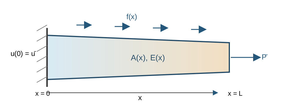
Under the one-dimensional bar assumptions, the axial strain, stress, and resultant axial force are
\[ \varepsilon(x)=\frac{\dd u}{\dd x}, \qquad \sigma(x)=E(x)\varepsilon(x), \qquad N(x)=A(x)\sigma(x)=A(x)E(x)\frac{\dd u}{\dd x}. \tag{4.44}\]
We take forces and displacements in the positive \(x\)-direction as positive. Balance of axial force on every subinterval gives
\[ -\frac{\dd N}{\dd x}=f \qquad\text{in }(0,L). \tag{4.45}\]
Substitution of Equation 4.44 into Equation 4.45 gives the strong equation
\[ -\frac{\dd}{\dd x}\left(AE\frac{\dd u}{\dd x}\right)=f \qquad\text{in }(0,L). \tag{4.46}\]
Let \(\Gamma_u\) and \(\Gamma_t\) be disjoint subsets of the two endpoints \(\partial\Om=\{0,L\}\). The complete boundary-value problem is
\[ \left\{ \begin{aligned} -\frac{\dd}{\dd x}\left(AE\frac{\dd u}{\dd x}\right)&=f &&\text{in }(0,L),\\ u&=\overline u &&\text{on }\Gamma_u,\\ Nn&=\overline P &&\text{on }\Gamma_t, \end{aligned} \right. \tag{4.47}\]
where the outward unit normal is \(n=-1\) at \(x=0\) and \(n=1\) at \(x=L\). Thus \(Nn\) is the outward axial force at an endpoint. For example, \(N(L)=\overline P\) when the force is prescribed at the right endpoint.
The trial and test spaces are
\[ \mathcal U_{\overline u} =\{w\in H^1(0,L):w=\overline u\text{ on }\Gamma_u\}, \qquad \mathcal V_0 =\{v\in H^1(0,L):v=0\text{ on }\Gamma_u\}. \tag{4.48}\]
Multiplying Equation 4.46 by \(v\in\mathcal V_0\), integrating over \((0,L)\), and applying one-dimensional integration by parts gives
\[ \int_0^L AE\,u'v'\,\dd x =\int_0^L fv\,\dd x +\sum_{x\in\Gamma_t}\overline P(x)v(x). \tag{4.49}\]
Accordingly, the variational problem is
\[ \boxed{ \text{find }u\in\mathcal U_{\overline u} \quad\text{such that}\quad a_{\mathrm{bar}}(u,v)=\ell_{\mathrm{bar}}(v) \quad\forall v\in\mathcal V_0,} \tag{4.50}\]
where
\[ a_{\mathrm{bar}}(u,v)=\int_0^L AE\,u'v'\,\dd x, \qquad \ell_{\mathrm{bar}}(v)=\int_0^L fv\,\dd x +\sum_{x\in\Gamma_t}\overline P(x)v(x). \tag{4.51}\]
Exercise 4.6 (Variational form of an axial bar) Starting from Equation 4.47:
- multiply the differential equation by a test function \(v\) and integrate over \((0,L)\);
- apply integration by parts and write the endpoint term using the outward normal \(n\);
- use the prescribed-force condition on \(\Gamma_t\) and \(v=0\) on \(\Gamma_u\); and
- obtain Equation 4.50 and identify its trial and test spaces.
4.5 Finite deformation and hyperelasticity
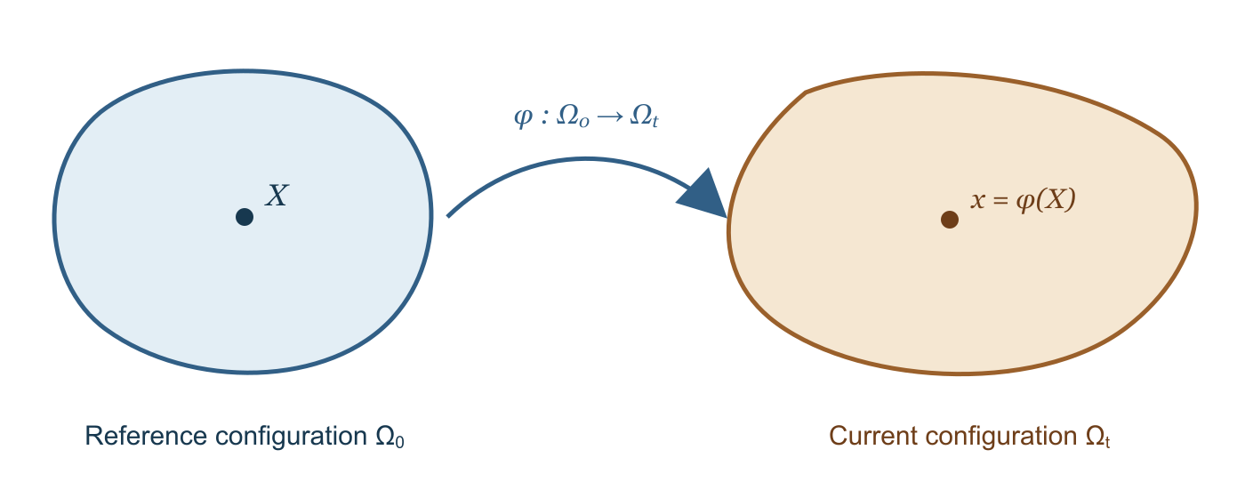
Small-strain kinematics are not appropriate when changes in length, angle, or orientation are large. We now distinguish reference and current configurations and formulate equilibrium over the reference body. Numerical linearization and solution are reserved for Chapter 10.
Figure 4.2 shows the two configurations and the deformation map between them.
4.5.1 Reference and current configurations
Let the reference configuration \(\Om_0\subset\R^d\) be a bounded Lipschitz domain. A material point is labeled by \(\bX\in\Om_0\). Reference position \(\bX\), current position \(\bx\), and displacement \(\bu\) are measured in meters. Throughout the finite-deformation formulation, uppercase \(\Grad\) and \(\Div\) denote differentiation with respect to the reference coordinate \(\bX\). For a vector field \(\bm w\) and a second-order tensor field \(\bm A\),
\[ (\Grad\bm w)_{iJ}=\frac{\partial w_i}{\partial X_J}, \qquad (\Div\bm A)_i=\frac{\partial A_{iJ}}{\partial X_J}. \tag{4.52}\]
The uppercase index \(J\) identifies a reference-coordinate direction, while the lowercase index \(i\) identifies a component in the current coordinate system. The deformation map
\[ \bm{\varphi}:\Om_0\to\Om_t, \qquad \bx=\bm{\varphi}(\bX)=\bX+\bu(\bX) \tag{4.53}\]
sends it to its current position \(\bx\in\Om_t\). The deformation gradient is
\[ \bF =\Grad\bm{\varphi} =\bI+\Grad\bu, \qquad F_{iJ}=\frac{\partial x_i}{\partial X_J}. \tag{4.54}\]
It maps an infinitesimal reference line element to its current counterpart:
\[ \dd\bx=\bF\,\dd\bX. \tag{4.55}\]
The Jacobian and right Cauchy–Green tensor are
\[ J=\det\bF, \qquad \bC=\bF^T\bF. \tag{4.56}\]
The tensors \(\bF\) and \(\bC\), and the scalar \(J\), are dimensionless. An admissible deformation must satisfy \(J>0\): the deformation must preserve orientation and cannot collapse a volume element to zero. Reference and current volume elements are related by
\[ \dd V_t=J\,\dd V_0. \tag{4.57}\]
Using Equation 4.55, the squared length of a reference line element after deformation is
\[ \dd\bx\cdot\dd\bx =\dd\bX\cdot\bC\,\dd\bX. \]
Its change in squared length is therefore
\[ \dd\bx\cdot\dd\bx-\dd\bX\cdot\dd\bX =\dd\bX\cdot(\bC-\bI)\,\dd\bX. \]
This relation motivates the Green–Lagrange strain tensor
\[ \bm{E} =\frac12(\bC-\bI) =\frac12\left( \Grad\bu+(\Grad\bu)^T+(\Grad\bu)^T\Grad\bu \right). \tag{4.58}\]
The strain \(\bm E\) is dimensionless. When the components of \(\Grad\bu\) are small, the quadratic term \((\Grad\bu)^T\Grad\bu\) can be neglected and \(\bm E\) reduces to the infinitesimal strain in Equation 4.17. At finite deformation, that quadratic term is retained. A rigid motion \(\bm{\varphi}(\bX)=\bm{Q}\bX+\bm{c}\), with \(\bm{Q}^T\bm{Q}=\bI\) and \(\det\bm{Q}=1\), gives \(\bC=\bI\) and \(\bm{E}=\bm{0}\).
Example 4.3 (Homogeneous stretch) For
\[ \bm{\varphi}(\bX)= \begin{bmatrix} \lambda_1X_1\\ \lambda_2X_2\\ \lambda_3X_3 \end{bmatrix}, \]
\[ \bF=\operatorname{diag}(\lambda_1,\lambda_2,\lambda_3), \quad J=\lambda_1\lambda_2\lambda_3, \quad \bC=\operatorname{diag}(\lambda_1^2,\lambda_2^2,\lambda_3^2). \]
Thus \(J\) is the local volume ratio and \(\bC\) records the squared principal stretches.
4.5.2 Stress measures and reference equilibrium
The Cauchy stress \(\bsig\) acts on current area. For a formulation over \(\Om_0\), use the first Piola–Kirchhoff stress
\[ \bP=J\bsig\bF^{-T}. \tag{4.59}\]
Both \(\bsig\) and \(\bP\) have units of pascals, but they refer to different areas. If corresponding current and reference area elements are denoted by \(\dd a\) and \(\dd A\), the stress transformation ensures that the same force is represented by \(\bsig\bn\,\dd a=\bP\bm N\,\dd A\). Thus the traction per unit reference area is \(\bP\bm{N}\), where \(\bm{N}\) is the outward unit normal to \(\partial\Om_0\). Although \(\bsig\) is symmetric, \(\bP\) is generally not symmetric because it relates current force components to reference area.
Let \(\bb_0\), measured in \(\mathrm{N}/\mathrm{m}^3\), be body force per unit reference volume. Consider an arbitrary subdomain \(\omega_0\subset\Om_0\). For quasistatic equilibrium, the total body and surface forces on \(\omega_0\) must sum to zero:
\[ \int_{\omega_0}\bb_0\,\dd V +\int_{\partial\omega_0}\bP\bm N\,\dd A =\bm 0. \tag{4.60}\]
Apply the tensor divergence theorem Equation 2.36 to the surface-force term in Equation 4.60. With \(\bm A=\bP\) and \(\omega=\omega_0\), the theorem gives
\[ \int_{\partial\omega_0}\bP\bm N\,\dd A =\int_{\omega_0}\Div\bP\,\dd V. \tag{4.61}\]
Substituting this result into Equation 4.60 gives the single volume integral
\[ \int_{\omega_0}(\Div\bP+\bb_0)\,\dd V=\bm 0. \]
Because this equation holds for every \(\omega_0\subset\Om_0\), localization gives \(-\Div\bP=\bb_0\) in \(\Om_0\).
Let \(\Gam_{0u}\) and \(\Gam_{0t}\) be relatively open, disjoint portions whose closures cover \(\partial\Om_0\). Displacement is prescribed on \(\Gam_{0u}\), and reference traction is prescribed on \(\Gam_{0t}\). The strong problem is
\[ \left. \begin{aligned} -\Div\bP&=\bb_0&&\text{in }\Om_0,\\ \bu&=\overline{\bu}&&\text{on }\Gam_{0u},\\ \bP\bm{N}&=\overline{\bt}_0&&\text{on }\Gam_{0t}. \end{aligned} \right\} \qquad\text{Strong form} \tag{4.62}\]
In components, Equation 4.62 is
\[ \left. \begin{aligned} -\frac{\partial P_{iJ}}{\partial X_J}&=b_{0i} &&\text{in }\Om_0,\\ u_i&=\overline u_i&&\text{on }\Gam_{0u},\\ P_{iJ}N_J&=\overline t_{0i}&&\text{on }\Gam_{0t}, \end{aligned} \right\} \qquad i=1,\ldots,d. \tag{4.63}\]
The repeated reference index \(J\) is summed, while \(i\) identifies the spatial component of the equilibrium equation.
4.5.3 Hyperelastic constitutive response
A hyperelastic material is defined by a stored-energy density \(\Psi(\bF)\) per unit reference volume, measured in \(\mathrm{J}/\mathrm{m}^3=\mathrm{Pa}\). For a fixed deformation gradient \(\bF\) and an arbitrary tensor \(\bm H\), the directional derivative of the energy density is
\[ \left.\frac{\dd}{\dd\epsilon} \Psi(\bF+\epsilon\bm H)\right|_{\epsilon=0} =\bP(\bF):\bm H. \tag{4.64}\]
Thus the first Piola–Kirchhoff stress is the derivative of \(\Psi\) with respect to \(\bF\):
\[ \bP=\frac{\partial\Psi}{\partial\bF}. \tag{4.65}\]
The existence of \(\Psi\) means that the stress work can be obtained from a stored energy. Now superpose a rigid rotation \(\bm Q\) on the current configuration. The deformation gradient changes from \(\bF\) to \(\bm Q\bF\), where \(\bm Q^T\bm Q=\bI\) and \(\det\bm Q=1\). A rigid rotation must not change the stored energy, so material frame indifference requires
\[ \Psi(\bm{Q}\bF)=\Psi(\bF). \]
For an isotropic material, the energy may be written in terms of scalar quantities that are unchanged by a change of orthonormal basis, such as \(\tr\bC\) and \(J\) (Belytschko et al. 2000; Bonet and Wood 2008).
A common compressible neo-Hookean model is
\[ \Psi(\bF) =\frac{\mu}{2}\bigl(\tr\bC-d\bigr) -\mu\ln J +\frac{\lambda}{2}(\ln J)^2, \qquad J>0. \tag{4.66}\]
The derivative identities
\[ \frac{\partial\,\tr\bC}{\partial\bF}=2\bF, \qquad \frac{\partial\ln J}{\partial\bF}=\bF^{-T} \]
give the corresponding first Piola–Kirchhoff stress
\[ \bP =\mu\left(\bF-\bF^{-T}\right) +\lambda(\ln J)\bF^{-T}. \tag{4.67}\]
Chapter 10 differentiates \(\bP\) with respect to \(\bF\) when constructing Newton’s method for the nonlinear equilibrium equations.
4.5.4 Reference-configuration variational problem
Using the same notation as in the small-strain problem, define the trial and test spaces over the reference configuration by
\[ \begin{aligned} \mathcal U_{\overline{\bu}} &=\{\bm{w}\in H^1(\Om_0;\R^d): \bm{w}=\overline{\bu}\text{ on }\Gam_{0u}\},\\ \mathcal V_0 &=\{\bv\in H^1(\Om_0;\R^d): \bv=\bm{0}\text{ on }\Gam_{0u}\}. \end{aligned} \tag{4.68}\]
Remark 4.6 (Admissible deformations). A finite deformation must also satisfy \(J>0\), and the stored-energy integral must be finite. In this chapter, we assume that the displacement sought in \(\mathcal U_{\overline{\bu}}\) satisfies these requirements. The function spaces and additional conditions used in a rigorous existence theory for nonlinear elasticity are outside the scope of this book.
To derive the variational form, let \(\bv\in\mathcal V_0\). Take the dot product of the equilibrium equation \(-\Div\bP=\bb_0\) with \(\bv\) and integrate over \(\Om_0\):
\[ -\int_{\Om_0}(\Div\bP)\cdot\bv\,\dd V =\int_{\Om_0}\bb_0\cdot\bv\,\dd V. \]
Tensor integration by parts gives
\[ \int_{\Om_0}\bP:\Grad\bv\,\dd V -\int_{\partial\Om_0}(\bP\bm N)\cdot\bv\,\dd A =\int_{\Om_0}\bb_0\cdot\bv\,\dd V. \tag{4.69}\]
The boundary integral is zero on \(\Gam_{0u}\) because \(\bv=\bm 0\). On \(\Gam_{0t}\), use \(\bP\bm N=\overline{\bt}_0\). Because the stress depends on the displacement through \(\bF(\bu)=\bI+\Grad\bu\), the variational problem is
\[ \left. \begin{aligned} &\text{Find }\bu\in\mathcal U_{\overline{\bu}}\text{ such that}\\ &\int_{\Om_0} \bP\bigl(\bF(\bu)\bigr):\Grad\bv\,\dd V = \int_{\Om_0}\bb_0\cdot\bv\,\dd V +\int_{\Gam_{0t}}\overline{\bt}_0\cdot\bv\,\dd A\\ &\hspace{17em}\forall\bv\in\mathcal V_0. \end{aligned} \right\} \qquad\text{Variational form} \tag{4.70}\]
In components, the variational equation is the scalar relation
\[ \int_{\Om_0} P_{iJ}\bigl(\bF(\bu)\bigr) \frac{\partial v_i}{\partial X_J}\,\dd V =\int_{\Om_0}b_{0i}v_i\,\dd V +\int_{\Gam_{0t}}\overline t_{0i}v_i\,\dd A. \tag{4.71}\]
Both \(i\) and \(J\) are repeated and summed.
To use the abstract notation of Chapter 3, define the internal semilinear form \(a_{\mathrm{hyp}}\) and the external load functional \(\ell_{\mathrm{hyp}}\) by
\[ \begin{aligned} a_{\mathrm{hyp}}(\bu;\bv) &=\int_{\Om_0} \bP\bigl(\bF(\bu)\bigr):\Grad\bv\,\dd V,\\ \ell_{\mathrm{hyp}}(\bv) &=\int_{\Om_0}\bb_0\cdot\bv\,\dd V +\int_{\Gam_{0t}}\overline{\bt}_0\cdot\bv\,\dd A. \end{aligned} \tag{4.72}\]
The compact statement of the variational problem is
\[ \left. \begin{aligned} &\text{Find }\bu\in\mathcal U_{\overline{\bu}}\text{ such that}\\ &a_{\mathrm{hyp}}(\bu;\bv)=\ell_{\mathrm{hyp}}(\bv) \qquad\forall\bv\in\mathcal V_0. \end{aligned} \right\} \qquad\text{Variational form} \tag{4.73}\]
The dependence of \(\bP\) on \(\bF(\bu)\) makes \(a_{\mathrm{hyp}}\) generally nonlinear in \(\bu\). For a fixed \(\bu\), it is linear in \(\bv\). It is therefore a semilinear form in the sense of Definition 2.24.
4.5.5 Total potential energy and equilibrium
The strong and variational equations are nonlinear in \(\bu\), but this does not prevent them from having an energy structure. For a hyperelastic material, \(\bP=\partial\Psi/\partial\bF\), so the internal semilinear form is the first variation of the stored energy. If \(\bb_0\) and \(\overline{\bt}_0\) are prescribed independently of the displacement, their external work also has a potential. Under these assumptions, define the total potential energy by
\[ \begin{aligned} \Pi_{\mathrm{hyp}}(\bm{w}) ={}&\int_{\Om_0}\Psi\bigl(\bF(\bm{w})\bigr)\,\dd V -\int_{\Om_0}\bb_0\cdot\bm{w}\,\dd V\\ &-\int_{\Gam_{0t}}\overline{\bt}_0\cdot\bm{w}\,\dd A, \qquad \bm w\in\mathcal U_{\overline{\bu}}. \end{aligned} \tag{4.74}\]
For a test function \(\bv\in\mathcal V_0\), perturb the displacement as \(\bu+\epsilon\bv\). The corresponding deformation gradient satisfies
\[ \bF(\bu+\epsilon\bv) =\bF(\bu)+\epsilon\Grad\bv, \]
and therefore \(\delta\bF(\bu;\bv)=\Grad\bv\). Applying the chain rule and Equation 4.64 to each term in Equation 4.74 gives
\[ \begin{aligned} \delta\Pi_{\mathrm{hyp}}(\bu;\bv) ={}& \int_{\Om_0} \bP\bigl(\bF(\bu)\bigr):\Grad\bv\,\dd V\\ &-\int_{\Om_0}\bb_0\cdot\bv\,\dd V -\int_{\Gam_{0t}}\overline{\bt}_0\cdot\bv\,\dd A. \end{aligned} \tag{4.75}\]
The stationarity condition \(\delta\Pi_{\mathrm{hyp}}(\bu;\bv)=0\) for every \(\bv\in\mathcal V_0\) is exactly the variational problem Equation 4.70. Thus, under the assumptions stated above, the equilibrium displacement can be obtained from either the variational problem or the stationarity of the total potential energy. Conditions under which a stationary point is a minimum, and questions of existence or uniqueness, are outside the scope of this chapter.
Exercise 4.7 (Deformation measures) For
\[ x_1=\lambda X_1+\gamma X_2, \qquad x_2=X_2, \]
- compute \(\bF\), \(J\), \(\bC\), and \(\bm{E}\);
- state the condition on \(\lambda\) required by \(J>0\); and
- identify the term in \(\bm{E}\) omitted by the small-strain approximation.
Exercise 4.8 (First variation of hyperelastic potential) Starting from Equation 4.74:
- use \(\bF(\bu+\epsilon\bv) =\bF(\bu)+\epsilon\Grad\bv\);
- apply the chain rule and \(\bP=\partial\Psi/\partial\bF\); and
- derive Equation 4.75 and then obtain the variational problem in Equation 4.70.
4.6 Common mathematical structure
Steady heat conduction and linear elasticity have the form
\[ \text{find }u\in\mathcal U_g \quad\text{such that}\quad a(u,v)=\ell(v) \qquad\forall v\in\mathcal V_0, \]
where \(a\) is bilinear. Temperature is scalar, while displacement and its test functions are vector-valued.
Transient heat conduction adds a capacity form
\[ m(\dot T,v)+a_T(T,v)=\ell_T(v), \qquad m(S,v)=\int_{\Om}\rho cSv\,\dx. \]
Hyperelasticity replaces the bilinear internal form by the semilinear form \(a_{\mathrm{hyp}}(\bu;\bv)\). The physical meanings must nevertheless be retained:
- \(k\grad T\) arises from energy balance and Fourier’s law;
- \(\mathbb C:\beps(\bu)\) arises from momentum balance, small-strain kinematics, and linear elasticity;
- \(\bP(\bF)\) acts on reference area and is derived from stored energy; and
- boundary signs depend on whether the prescribed quantity is an outward physical flux or the normal component used in an abstract equation.
Chapter 5 replaces the continuous spaces by finite-dimensional spaces. The physical models and continuous variational problems remain unchanged.
Exercise 4.9 (Comparing the model problems) For steady heat conduction, transient heat conduction, linear elasticity, and hyperelasticity, identify:
- the primary unknown;
- the balance law;
- the constitutive equation;
- the essential and natural boundary data; and
- whether the variational form is bilinear, semilinear, or contains a time derivative.
4.7 Chapter summary
- Energy balance and Fourier’s law give the transient heat equation. Removing the time derivative gives steady heat conduction.
- Prescribed temperature is essential boundary data. Prescribed outward heat flux is natural data, while convection produces a Robin term.
- Small-strain elasticity combines infinitesimal kinematics, balance of linear momentum, and a linear elastic constitutive equation.
- The principle of virtual work is the variational statement of quasistatic equilibrium and the stationarity condition of total potential energy.
- Finite-deformation kinematics distinguish reference and current configurations through the deformation map, \(\bF\), \(J\), and \(\bC\).
- Hyperelastic stress is derived from stored energy. The resulting reference-configuration variational form is nonlinear in displacement and linear in the test function.
- Similar variational structures allow the same finite element framework to treat different physics, but each form retains the meaning and sign conventions of its physical model.